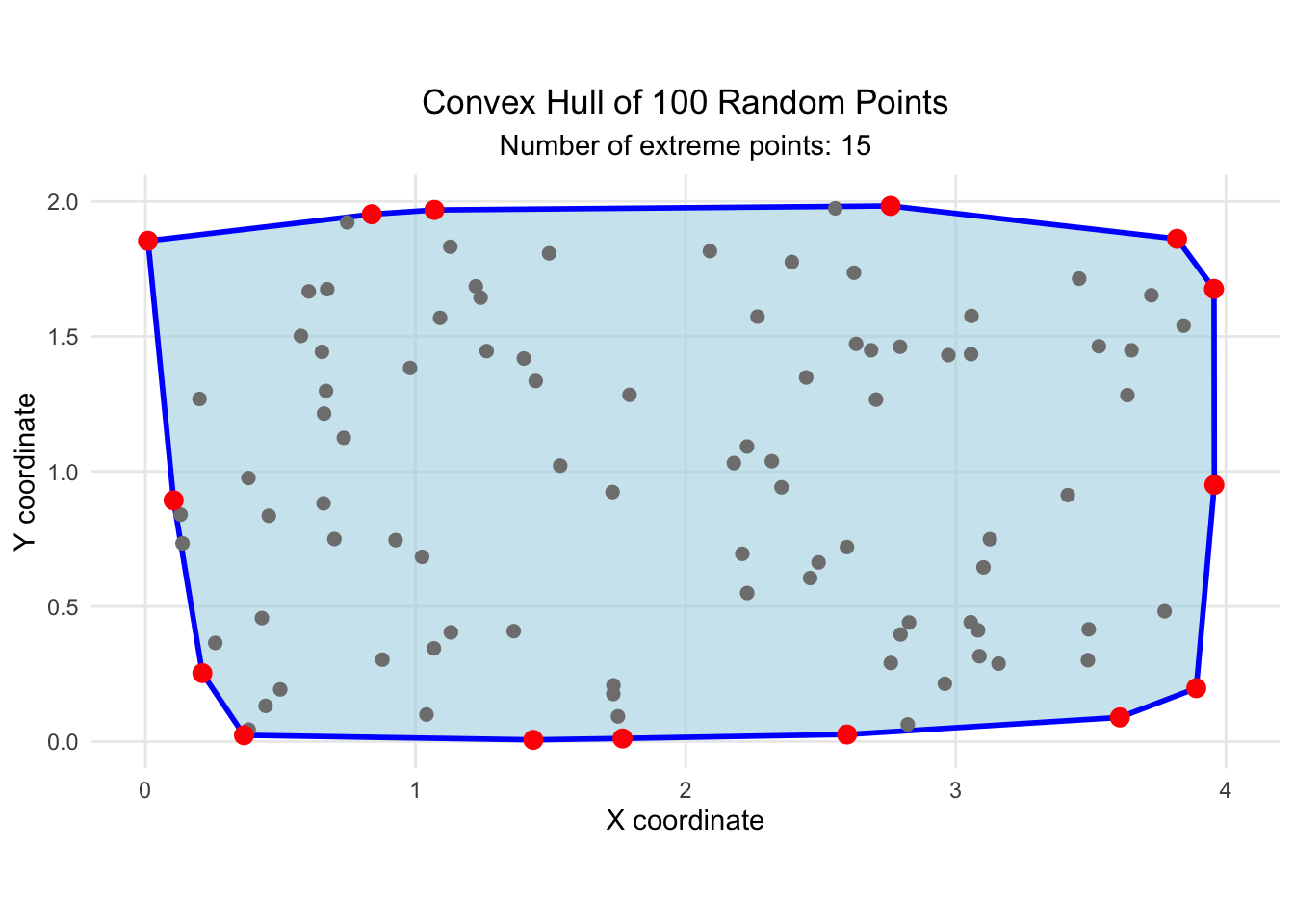
# Load required librarieslibrary(ggplot2)library(grDevices)# Set seed for reproducibilityset.seed(50720235)# Generate random uniform points in rectangle [0,4] by [0,2]n_points <-100# Number of random pointsx <-runif(n_points, min =0, max =4)y <-runif(n_points, min =0, max =2)# Create data framepoints_df <-data.frame(x = x, y = y)# Compute convex hullhull_indices <-chull(x, y)hull_points <- points_df[hull_indices, ]# Add first point at the end to close the polygonhull_points <-rbind(hull_points, hull_points[1, ])# Count extreme points (vertices of convex hull)n_extreme_points <-length(hull_indices)# Create the plotp <-ggplot() +# Add shaded convex hull region in light bluegeom_polygon(data = hull_points, aes(x = x, y = y), fill ="lightblue", alpha =0.6, color ="blue", linewidth =1) +# Add all random points in graygeom_point(data = points_df, aes(x = x, y = y), color ="gray50", size =2) +# Add extreme points (hull vertices) in redgeom_point(data = points_df[hull_indices, ], aes(x = x, y = y), color ="red", size =3) +# Formattingxlim(0, 4) +ylim(0, 2) +labs(title =paste("Convex Hull of", n_points, "Random Points"),subtitle =paste("Number of extreme points:", n_extreme_points),x ="X coordinate", y ="Y coordinate") +theme_minimal() +theme(panel.grid.minor =element_blank(),plot.title =element_text(hjust =0.5),plot.subtitle =element_text(hjust =0.5)) +coord_fixed() # Maintain aspect ratio# Display the plotprint(p)
Code
# Print summary informationcat("Summary:\n")
Summary:
Code
cat("Total points generated:", n_points, "\n")
Total points generated: 100
Code
cat("Number of extreme points (convex hull vertices):", n_extreme_points, "\n")
Number of extreme points (convex hull vertices): 15
Code
cat("Proportion of extreme points:", round(n_extreme_points/n_points, 3), "\n")
Proportion of extreme points: 0.15
Code
# Save the plot file (uncomment as necessary)# ggsave("convex_hull_plot.png", plot = p, width = 8, height = 6, units = "in")
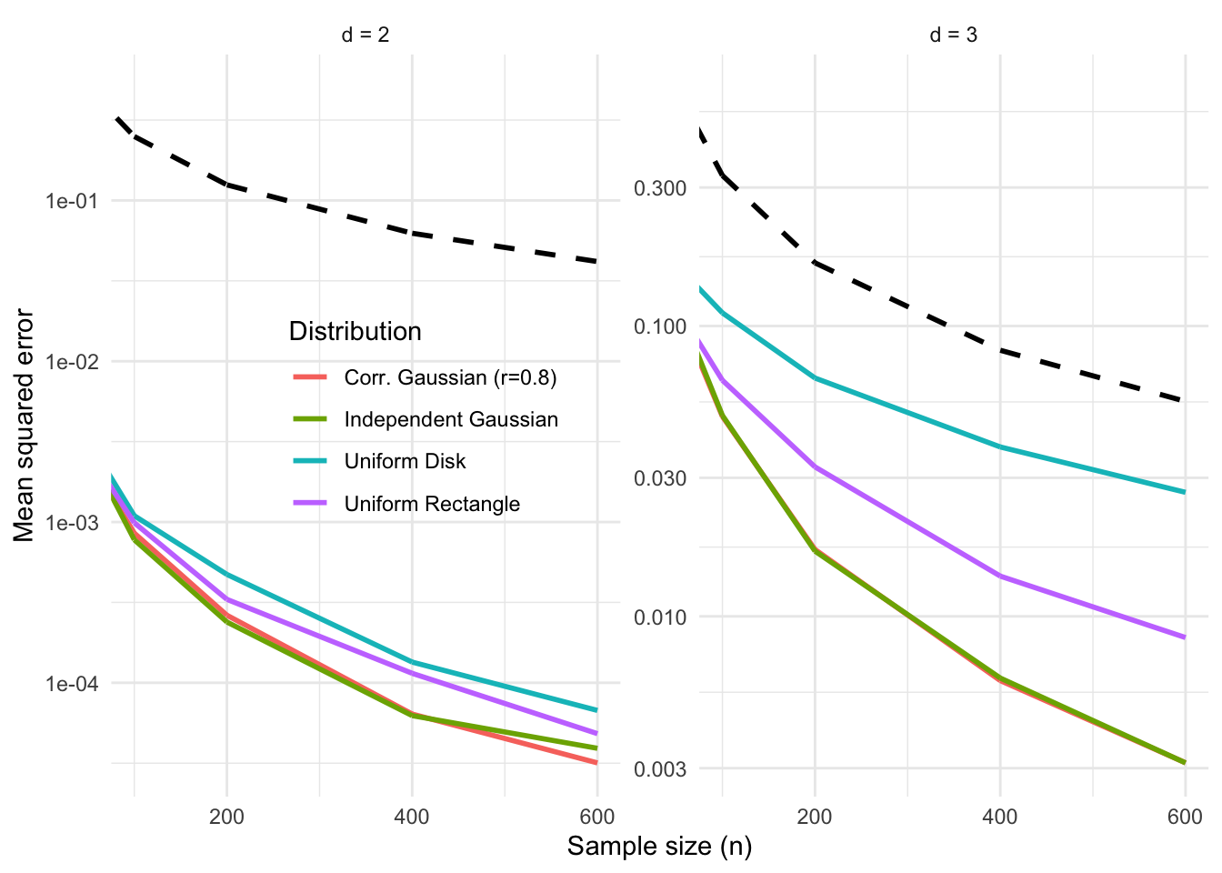
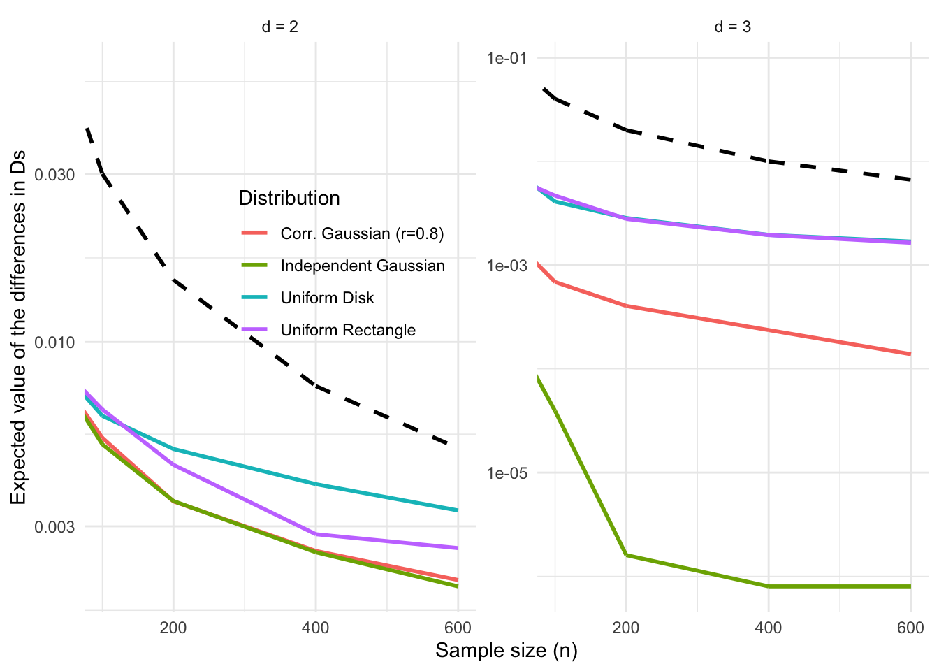
Code for Figures 2 and 3 that illustrate the theorem for different distributions
This shows the generation of the figures for the convex hull verifications in section 2.2. Added on is the case of uniform points on a disk.
Code
# Load required librarieslibrary(ggplot2)library(dplyr)library(gridExtra)library(geometry)library(MASS) # for mvrnormlibrary(sp) # for point.in.polygon
Code
# Generate points from uniform distribution on a diskgenerate_uniform_disk_points <-function(n, d, radius =1) {if (d !=2) {stop("Uniform disk distribution is only implemented for d = 2") }# Generate angles uniformly between 0 and 2π theta <-runif(n, 0, 2*pi)# Generate radii with r ~ sqrt(U) for uniformity# (in 2D, need r ~ U^(1/2) for uniform distribution in disk) r <- radius *sqrt(runif(n))# Convert to Cartesian coordinates x <- r *cos(theta) y <- r *sin(theta)return(cbind(x, y))}
Generation functions for different distributions
Code
# Function to generate points from different distributionsgenerate_distribution_points <-function(n, d, distribution, correlation =0.5) {if(distribution =="uniform_rectangle") {# Uniform in [0,4] x [0,2] (only for d=2) or [0,4] x [0,2] x [0,1] (for d=3)if(d ==2) { X <-cbind(runif(n, 0, 4), runif(n, 0, 2)) } elseif(d ==3) { X <-cbind(runif(n, 0, 4), runif(n, 0, 2), runif(n, 0, 1)) } } elseif (distribution =="uniform_disk") {# Uniform distribution on diskif(d ==2) {# 2D disk implementation theta <-runif(n, 0, 2*pi) r <-sqrt(runif(n)) x <- r *cos(theta) y <- r *sin(theta)return(cbind(x, y)) } elseif(d ==3) {# 3D ball implementation# Generate points from a 3D ball using spherical coordinates theta <-runif(n, 0, 2*pi) # Azimuthal angle phi <-acos(2*runif(n) -1) # Polar angle r <-runif(n)^(1/3) # Radius (cube root for uniform distribution) x <- r *sin(phi) *cos(theta) y <- r *sin(phi) *sin(theta) z <- r *cos(phi)return(cbind(x, y, z)) } } elseif(distribution =="gaussian_independent") {# Independent standard Gaussians X <-matrix(rnorm(n * d, 0, 1), ncol = d) } elseif(distribution =="gaussian_correlated") {# Correlated Gaussians with correlation r Sigma <-matrix(correlation, nrow = d, ncol = d)diag(Sigma) <-1 X <-mvrnorm(n, mu =rep(0, d), Sigma = Sigma) }return(X)}
Estimate Dn by Monte Carlo
Code
# Function to estimate D_n using Monte Carloestimate_D_n <-function(hull_points, distribution, d, correlation =0.5, n_test =5000) {# Generate test points from the same distribution test_points <-generate_distribution_points(n_test, d, distribution, correlation)if(d ==2) {# Use point.in.polygon for 2Dif(nrow(hull_points) <3) return(1) # If no proper hull, D_n = 1# Ensure hull is closedif(!all(hull_points[1,] == hull_points[nrow(hull_points),])) { hull_points <-rbind(hull_points, hull_points[1,]) } inside_count <-sum(point.in.polygon(test_points[,1], test_points[,2], hull_points[,1], hull_points[,2]) >0) D_n <-1- inside_count / n_test } elseif(d ==3) {# Simple approximation for 3D using bounding boxif(nrow(hull_points) <4) return(1) bbox_min <-apply(hull_points, 2, min) bbox_max <-apply(hull_points, 2, max)# Count points inside bounding box (conservative approximation) inside_bbox <-apply(test_points, 1, function(pt) {all(pt >= bbox_min) &&all(pt <= bbox_max) })# For Gaussian distributions, estimate the total "relevant" measureif(distribution =="uniform_rectangle") { total_measure <-4*2*1# [0,4] x [0,2] x [0,1] inside_count <-sum(inside_bbox) D_n <-1- inside_count / n_test } elseif(distribution =="uniform_disk") {# For uniform disk, same approach as above inside_count <-sum(inside_bbox) D_n <-1- inside_count / n_test } else {# For Gaussians, use a more conservative estimate# Assume most probability mass is within some reasonable bounds center <-colMeans(hull_points) inside_count <-sum(apply(test_points, 1, function(pt) {sqrt(sum((pt - center)^2)) <=0.6*sqrt(sum((bbox_max - bbox_min)^2)) })) D_n <-1- inside_count / n_test } }return(max(0, min(1, D_n))) # Clamp to [0,1]}
Illustration of the main theorem
Code
# Main simulation function for the theoremsimulate_main_theorem <-function(n, d, distribution, correlation =0.5, n_simulations =300) { results <-data.frame(simulation =integer(n_simulations),V_n =integer(n_simulations),D_n =numeric(n_simulations),D_n_minus_1 =numeric(n_simulations),V_n_over_n =numeric(n_simulations),difference_squared =numeric(n_simulations),D_diff =numeric(n_simulations),n =integer(n_simulations),d =integer(n_simulations),distribution =character(n_simulations),stringsAsFactors =FALSE )for(i in1:n_simulations) {# Generate n points X_n <-generate_distribution_points(n, d, distribution, correlation)# Generate n-1 points for D_{n-1} X_n_minus_1 <- X_n[1:(n-1), ]# Compute convex hullsif(d ==2) {# For n points hull_indices_n <-chull(X_n[,1], X_n[,2]) V_n <-length(hull_indices_n) hull_points_n <- X_n[hull_indices_n, ]# For n-1 points hull_indices_n_minus_1 <-chull(X_n_minus_1[,1], X_n_minus_1[,2]) hull_points_n_minus_1 <- X_n_minus_1[hull_indices_n_minus_1, ] } elseif(d ==3) {# For n points hull_faces_n <-convhulln(X_n, options ="Pp") V_n <-length(unique(as.vector(hull_faces_n))) hull_vertices_n <- X_n[unique(as.vector(hull_faces_n)), ]# For n-1 points hull_faces_n_minus_1 <-convhulln(X_n_minus_1, options ="Pp") hull_vertices_n_minus_1 <- X_n_minus_1[unique(as.vector(hull_faces_n_minus_1)), ] }# Estimate D_n and D_{n-1}if(d ==2) { D_n <-estimate_D_n(hull_points_n, distribution, d, correlation) D_n_minus_1 <-estimate_D_n(hull_points_n_minus_1, distribution, d, correlation) } else { D_n <-estimate_D_n(hull_vertices_n, distribution, d, correlation) D_n_minus_1 <-estimate_D_n(hull_vertices_n_minus_1, distribution, d, correlation) }# Compute the quantities in the theorem V_n_over_n <- V_n / n difference_squared <- (V_n_over_n - D_n_minus_1)^2 D_diff <-abs(D_n - D_n_minus_1) results[i, ] <-list(i, V_n, D_n, D_n_minus_1, V_n_over_n, difference_squared, D_diff, n, d, distribution)#if(i %% 50 == 0) cat("Completed", i, "of", n_simulations, "simulations\n") }return(results)}
Run simulations for sample sizes from 50 to 600.
Code
# Set seed for reproducibilityset.seed(20421)# Simulation parameterssample_sizes <-c(50, 100, 200, 400, 600)dimensions <-c(2, 3)distributions <-c("uniform_rectangle", "uniform_disk", "gaussian_independent", "gaussian_correlated")correlation <-0.8n_sims <-250#cat("Running main theorem simulations...\n")# Run all simulationsall_theorem_data <-data.frame()for(d in dimensions) {for(dist in distributions) {for(n in sample_sizes) {#cat("\n--- Running", dist, "d =", d, "n =", n, "---\n") sim_data <-simulate_main_theorem(n, d, dist, correlation, n_sims) all_theorem_data <-rbind(all_theorem_data, sim_data) } }}# Clean up distribution labelsall_theorem_data$distribution_clean <-case_when( all_theorem_data$distribution =="uniform_rectangle"~"Uniform Rectangle", all_theorem_data$distribution =="uniform_disk"~"Uniform Disk", all_theorem_data$distribution =="gaussian_independent"~"Independent Gaussian", all_theorem_data$distribution =="gaussian_correlated"~paste0("Corr. Gaussian (r=", correlation, ")"),TRUE~ all_theorem_data$distribution)cat("\nSimulations complete. Creating plots...\n")
Supplementary plot of theoretical versus estimates
Code
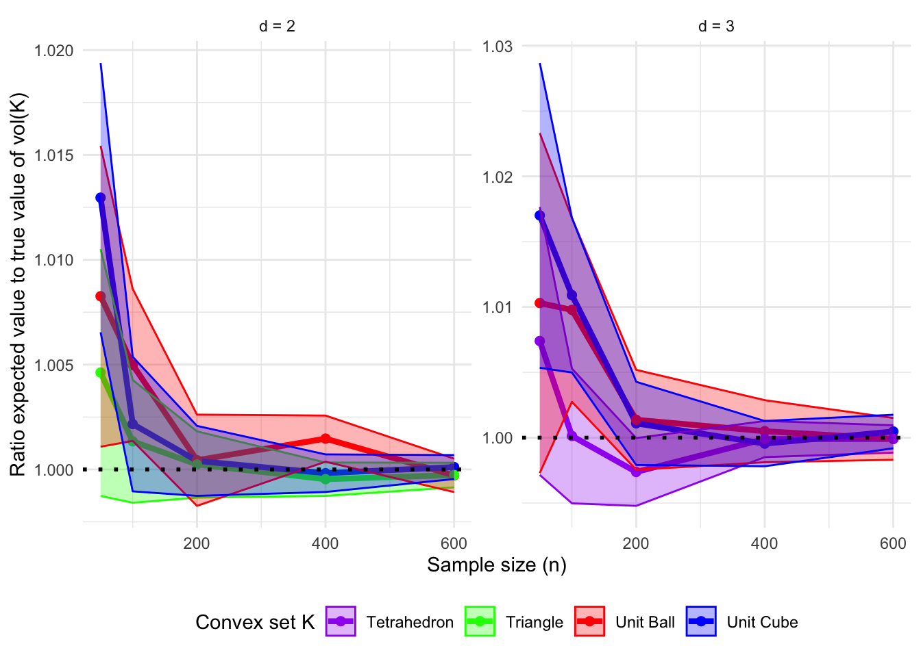
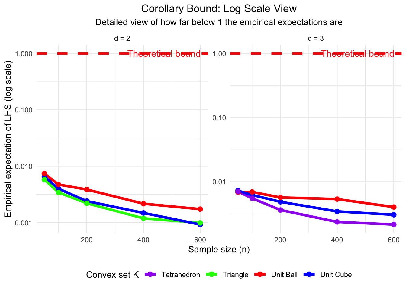
# Print summary resultscat("\n=== COROLLARY VERIFICATION WITH SIMPLEX ===\n")cat("Theoretical bound: E[LHS] ≤ 1\n\n")summary_table <- summary_data %>%select(K_type_clean, d, n, empirical_expectation, prop_exceed_1) %>%arrange(d, K_type_clean, n)print(summary_table)cat("\nMaximum empirical expectation by case:\n")max_by_case <- summary_data %>%group_by(K_type_clean, d) %>%summarise(max_empirical_exp =max(empirical_expectation),min_n_for_max = n[which.max(empirical_expectation)],avg_empirical_exp =mean(empirical_expectation),.groups ='drop' )print(max_by_case)cat("\nVolume estimator performance (bias from 1):\n")vol_bias <- vol_estimator_data %>%group_by(K_type_clean, d) %>%summarise(avg_bias =mean(mean_vol_ratio -1),max_bias =max(abs(mean_vol_ratio -1)),.groups ='drop' )print(vol_bias)cat("\nCases where empirical expectation > 1:\n")violations <- summary_data[summary_data$empirical_expectation >1, ]if(nrow(violations) >0) {print(violations[, c("K_type_clean", "d", "n", "empirical_expectation")])} else {cat("None! The bound holds in all cases.\n")}cat("\n=== SUMMARY ===\n")cat("All empirical expectations are smaller than 1, suggesting the bound is quite conservative.\n")cat("The tetrahedron (4-simplex in 3D) case has been added.\n")cat("Volume estimator shows good performance across all convex sets.\n")
The tetrahedron case uses the standard 3-simplex with vertices at (0,0,0), (1,0,0), (0,1,0), (0,0,1) and generates uniform points using the Dirichlet distribution method.
The LHS values being quite smaller than 1 suggests the theoretical bound is quite conservative.
Source Code
---title: "Convex Hull Theorem Illustration"subtitle: "Figures 1-4"execute: warning: false message: false cache: false---## A convex hull with 100 points (Figure 1)```{r example}# Load required librarieslibrary(ggplot2)library(grDevices)# Set seed for reproducibilityset.seed(50720235)# Generate random uniform points in rectangle [0,4] by [0,2]n_points <- 100 # Number of random pointsx <- runif(n_points, min = 0, max = 4)y <- runif(n_points, min = 0, max = 2)# Create data framepoints_df <- data.frame(x = x, y = y)# Compute convex hullhull_indices <- chull(x, y)hull_points <- points_df[hull_indices, ]# Add first point at the end to close the polygonhull_points <- rbind(hull_points, hull_points[1, ])# Count extreme points (vertices of convex hull)n_extreme_points <- length(hull_indices)# Create the plotp <- ggplot() + # Add shaded convex hull region in light blue geom_polygon(data = hull_points, aes(x = x, y = y), fill = "lightblue", alpha = 0.6, color = "blue", linewidth = 1) + # Add all random points in gray geom_point(data = points_df, aes(x = x, y = y), color = "gray50", size = 2) + # Add extreme points (hull vertices) in red geom_point(data = points_df[hull_indices, ], aes(x = x, y = y), color = "red", size = 3) + # Formatting xlim(0, 4) + ylim(0, 2) + labs(title = paste("Convex Hull of", n_points, "Random Points"), subtitle = paste("Number of extreme points:", n_extreme_points), x = "X coordinate", y = "Y coordinate") + theme_minimal() + theme(panel.grid.minor = element_blank(), plot.title = element_text(hjust = 0.5), plot.subtitle = element_text(hjust = 0.5)) + coord_fixed() # Maintain aspect ratio# Display the plotprint(p)# Print summary informationcat("Summary:\n")cat("Total points generated:", n_points, "\n")cat("Number of extreme points (convex hull vertices):", n_extreme_points, "\n")cat("Proportion of extreme points:", round(n_extreme_points/n_points, 3), "\n")# Save the plot file (uncomment as necessary)# ggsave("convex_hull_plot.png", plot = p, width = 8, height = 6, units = "in")```## Code for Figures 2 and 3 that illustrate the theorem for different distributions This shows the generation of the figures for the convex hull verifications in section 2.2.Added on is the case of uniform points on a disk.```{r setup}# Load required librarieslibrary(ggplot2)library(dplyr)library(gridExtra)library(geometry)library(MASS) # for mvrnormlibrary(sp) # for point.in.polygon``````{r uniformdisk, eval=FALSE}# Generate points from uniform distribution on a diskgenerate_uniform_disk_points <- function(n, d, radius = 1) { if (d != 2) { stop("Uniform disk distribution is only implemented for d = 2") } # Generate angles uniformly between 0 and 2π theta <- runif(n, 0, 2*pi) # Generate radii with r ~ sqrt(U) for uniformity # (in 2D, need r ~ U^(1/2) for uniform distribution in disk) r <- radius * sqrt(runif(n)) # Convert to Cartesian coordinates x <- r * cos(theta) y <- r * sin(theta) return(cbind(x, y))}```## Generation functions for different distributions```{r distributions}#| code-fold: TRUE# Function to generate points from different distributionsgenerate_distribution_points <- function(n, d, distribution, correlation = 0.5) { if(distribution == "uniform_rectangle") { # Uniform in [0,4] x [0,2] (only for d=2) or [0,4] x [0,2] x [0,1] (for d=3) if(d == 2) { X <- cbind(runif(n, 0, 4), runif(n, 0, 2)) } else if(d == 3) { X <- cbind(runif(n, 0, 4), runif(n, 0, 2), runif(n, 0, 1)) } } else if (distribution == "uniform_disk") { # Uniform distribution on disk if(d == 2) { # 2D disk implementation theta <- runif(n, 0, 2*pi) r <- sqrt(runif(n)) x <- r * cos(theta) y <- r * sin(theta) return(cbind(x, y)) } else if(d == 3) { # 3D ball implementation # Generate points from a 3D ball using spherical coordinates theta <- runif(n, 0, 2*pi) # Azimuthal angle phi <- acos(2*runif(n) - 1) # Polar angle r <- runif(n)^(1/3) # Radius (cube root for uniform distribution) x <- r * sin(phi) * cos(theta) y <- r * sin(phi) * sin(theta) z <- r * cos(phi) return(cbind(x, y, z)) } } else if(distribution == "gaussian_independent") { # Independent standard Gaussians X <- matrix(rnorm(n * d, 0, 1), ncol = d) } else if(distribution == "gaussian_correlated") { # Correlated Gaussians with correlation r Sigma <- matrix(correlation, nrow = d, ncol = d) diag(Sigma) <- 1 X <- mvrnorm(n, mu = rep(0, d), Sigma = Sigma) } return(X)}```## Estimate Dn by Monte Carlo```{r MCDn}#| code-fold: TRUE# Function to estimate D_n using Monte Carloestimate_D_n <- function(hull_points, distribution, d, correlation = 0.5, n_test = 5000) { # Generate test points from the same distribution test_points <- generate_distribution_points(n_test, d, distribution, correlation) if(d == 2) { # Use point.in.polygon for 2D if(nrow(hull_points) < 3) return(1) # If no proper hull, D_n = 1 # Ensure hull is closed if(!all(hull_points[1,] == hull_points[nrow(hull_points),])) { hull_points <- rbind(hull_points, hull_points[1,]) } inside_count <- sum(point.in.polygon(test_points[,1], test_points[,2], hull_points[,1], hull_points[,2]) > 0) D_n <- 1 - inside_count / n_test } else if(d == 3) { # Simple approximation for 3D using bounding box if(nrow(hull_points) < 4) return(1) bbox_min <- apply(hull_points, 2, min) bbox_max <- apply(hull_points, 2, max) # Count points inside bounding box (conservative approximation) inside_bbox <- apply(test_points, 1, function(pt) { all(pt >= bbox_min) && all(pt <= bbox_max) }) # For Gaussian distributions, estimate the total "relevant" measure if(distribution == "uniform_rectangle") { total_measure <- 4 * 2 * 1 # [0,4] x [0,2] x [0,1] inside_count <- sum(inside_bbox) D_n <- 1 - inside_count / n_test } else if(distribution == "uniform_disk") { # For uniform disk, same approach as above inside_count <- sum(inside_bbox) D_n <- 1 - inside_count / n_test } else { # For Gaussians, use a more conservative estimate # Assume most probability mass is within some reasonable bounds center <- colMeans(hull_points) inside_count <- sum(apply(test_points, 1, function(pt) { sqrt(sum((pt - center)^2)) <= 0.6 * sqrt(sum((bbox_max - bbox_min)^2)) })) D_n <- 1 - inside_count / n_test } } return(max(0, min(1, D_n))) # Clamp to [0,1]}```## Illustration of the main theorem```{r mainthm}#| code-fold: TRUE# Main simulation function for the theoremsimulate_main_theorem <- function(n, d, distribution, correlation = 0.5, n_simulations = 300) { results <- data.frame( simulation = integer(n_simulations), V_n = integer(n_simulations), D_n = numeric(n_simulations), D_n_minus_1 = numeric(n_simulations), V_n_over_n = numeric(n_simulations), difference_squared = numeric(n_simulations), D_diff = numeric(n_simulations), n = integer(n_simulations), d = integer(n_simulations), distribution = character(n_simulations), stringsAsFactors = FALSE ) for(i in 1:n_simulations) { # Generate n points X_n <- generate_distribution_points(n, d, distribution, correlation) # Generate n-1 points for D_{n-1} X_n_minus_1 <- X_n[1:(n-1), ] # Compute convex hulls if(d == 2) { # For n points hull_indices_n <- chull(X_n[,1], X_n[,2]) V_n <- length(hull_indices_n) hull_points_n <- X_n[hull_indices_n, ] # For n-1 points hull_indices_n_minus_1 <- chull(X_n_minus_1[,1], X_n_minus_1[,2]) hull_points_n_minus_1 <- X_n_minus_1[hull_indices_n_minus_1, ] } else if(d == 3) { # For n points hull_faces_n <- convhulln(X_n, options = "Pp") V_n <- length(unique(as.vector(hull_faces_n))) hull_vertices_n <- X_n[unique(as.vector(hull_faces_n)), ] # For n-1 points hull_faces_n_minus_1 <- convhulln(X_n_minus_1, options = "Pp") hull_vertices_n_minus_1 <- X_n_minus_1[unique(as.vector(hull_faces_n_minus_1)), ] } # Estimate D_n and D_{n-1} if(d == 2) { D_n <- estimate_D_n(hull_points_n, distribution, d, correlation) D_n_minus_1 <- estimate_D_n(hull_points_n_minus_1, distribution, d, correlation) } else { D_n <- estimate_D_n(hull_vertices_n, distribution, d, correlation) D_n_minus_1 <- estimate_D_n(hull_vertices_n_minus_1, distribution, d, correlation) } # Compute the quantities in the theorem V_n_over_n <- V_n / n difference_squared <- (V_n_over_n - D_n_minus_1)^2 D_diff <- abs(D_n - D_n_minus_1) results[i, ] <- list(i, V_n, D_n, D_n_minus_1, V_n_over_n, difference_squared, D_diff, n, d, distribution) #if(i %% 50 == 0) cat("Completed", i, "of", n_simulations, "simulations\n") } return(results)}```## Run simulations for sample sizes from 50 to 600.```{r simulations}#| code-fold: true# Set seed for reproducibilityset.seed(20421)# Simulation parameterssample_sizes <- c(50, 100, 200, 400, 600)dimensions <- c(2, 3)distributions <- c("uniform_rectangle", "uniform_disk", "gaussian_independent", "gaussian_correlated")correlation <- 0.8n_sims <- 250#cat("Running main theorem simulations...\n")# Run all simulationsall_theorem_data <- data.frame()for(d in dimensions) { for(dist in distributions) { for(n in sample_sizes) { #cat("\n--- Running", dist, "d =", d, "n =", n, "---\n") sim_data <- simulate_main_theorem(n, d, dist, correlation, n_sims) all_theorem_data <- rbind(all_theorem_data, sim_data) } }}# Clean up distribution labelsall_theorem_data$distribution_clean <- case_when( all_theorem_data$distribution == "uniform_rectangle" ~ "Uniform Rectangle", all_theorem_data$distribution == "uniform_disk" ~ "Uniform Disk", all_theorem_data$distribution == "gaussian_independent" ~ "Independent Gaussian", all_theorem_data$distribution == "gaussian_correlated" ~ paste0("Corr. Gaussian (r=", correlation, ")"), TRUE ~ all_theorem_data$distribution)cat("\nSimulations complete. Creating plots...\n")# Compute summary statisticstheorem_summary <- all_theorem_data %>% group_by(distribution_clean, d, n) %>% summarise( mean_squared_diff = mean(difference_squared), theoretical_bound = (8*d + 9) / n, mean_D_diff = mean(D_diff), theoretical_D_bound = (d + 1) / n, mean_V_n_over_n = mean(V_n_over_n), mean_D_n_minus_1 = mean(D_n_minus_1), sd_squared_diff = sd(difference_squared), .groups = 'drop' )```## Creation of Figure 2```{r plot2}# FIGURE 2: Main theorem bound - MSEfig2 <- ggplot(theorem_summary, aes(x = n)) + geom_line(aes(y = mean_squared_diff, color = distribution_clean), size = 1) + geom_line(aes(y = theoretical_bound), linetype = "dashed", color = "black", size = 1) + facet_wrap(~paste("d =", d), scales = "free_y") + labs(x = "Sample size (n)", y = "Mean squared error", color = "Distribution") + theme_minimal() + theme(legend.position = c(0.15, 0.35), legend.justification = c("left","bottom"))+ coord_cartesian(xlim = c(100, max(theorem_summary$n)))+ scale_y_log10() #+ #+annotate("text", x = 400, y = 0.1, label = "Theoretical bound", # color = "black", size = 3)print(fig2)# ggsave("main_theorem_mse_bound.png", fig2, width = 7, height = 4,dpi = 300, bg = "white")```## Second part of theorem, Figure showing D_n difference```{r}# FIGURE 3: Second part of theorem - D_n differencefig3 <-ggplot(theorem_summary, aes(x = n)) +geom_line(aes(y = mean_D_diff, color = distribution_clean), linewidth =1) +geom_line(aes(y = theoretical_D_bound), linetype ="dashed", color ="black", size =1) +facet_wrap(~paste("d =", d), scales ="free_y") +labs(x ="Sample size (n)",y ="Expected value of the differences in Ds",color ="Distribution") +theme_minimal() +theme(legend.position =c(0.17,0.45),legend.justification =c("left","bottom"))+coord_cartesian(xlim =c(100, max(theorem_summary$n)))+scale_y_log10() #+# annotate("text", x = 400, y = 0.01, label = "Theoretical bound", # color = "black", size = 3)print(fig3)# To save to a file# ggsave("main_theorem_D_diff_bound.png", fig3, # width = 7, height = 4, dpi = 300, bg = "white")```## Convergence of expectations ```{r}# FIGURE 4: Convergence of expectationsfig4 <-ggplot(theorem_summary, aes(x = n)) +geom_line(aes(y = mean_V_n_over_n, color =paste(distribution_clean, expression(-V[n]/n))), size =1.5, alpha =0.7) +geom_line(aes(y = mean_D_n_minus_1, color =paste(distribution_clean, expression(-D[n-1]))), size =1.5, alpha =0.7) +facet_wrap(~paste("d =", d), scales ="free_y") +labs(#title = expression("Convergence: " * E[V[n]/n] * " and " * E[D[n-1]]),#subtitle = "The theorem states these should be equal in expectation",x ="Sample size (n)",y ="Expected value",color ="Quantity") +theme_minimal() +theme(legend.position ="bottom") +guides(color =guide_legend(ncol =2))print(fig4)#ggsave("main_theorem_convergence.png", fig4, # width = 6, height = 4, dpi = 300, bg = "white")# Print summary statisticscat("\n=== MAIN THEOREM VERIFICATION ===\n")print(theorem_summary)cat("\nBound violations for MSE:\n")mse_violations <- theorem_summary[theorem_summary$mean_squared_diff > theorem_summary$theoretical_bound, ]if(nrow(mse_violations) >0) {print(mse_violations[, c("distribution_clean", "d", "n", "mean_squared_diff", "theoretical_bound")])} else {cat("None! The MSE bound holds in all cases.\n")}cat("\nBound violations for D difference:\n")D_violations <- theorem_summary[theorem_summary$mean_D_diff > theorem_summary$theoretical_D_bound, ]if(nrow(D_violations) >0) {print(D_violations[, c("distribution_clean", "d", "n", "mean_D_diff", "theoretical_D_bound")])} else {cat("None! The D difference bound holds in all cases.\n")}cat("\nExpectation equality check (should be close to 0):\n")expectation_diff <- theorem_summary %>%mutate(expectation_difference =abs(mean_V_n_over_n - mean_D_n_minus_1)) %>%arrange(desc(expectation_difference))# Print just the relevant columnsprint(head(expectation_diff[, c("distribution_clean", "d", "n", "expectation_difference")], 10))cat("\n=== SUMMARY ===\n")cat("This code illustrates the main theorem with:\n")cat("1. MSE bound: E[(V_n/n - D_{n-1})^2] ≤ (8d+10)/n\n")cat("2. D difference bound: E[|D_n - D_{n-1}|] ≤ (d+1)/n\n")cat("3. Expectation equality: E[V_n/n] = E[D_{n-1}]\n")cat("4. Three distributions across 2D and 3D\n")```## Corollary Illustration with creation of Fig 4```{r}# Load required librarieslibrary(ggplot2)library(dplyr)library(gridExtra)library(geometry)# Function to simulate the corollary bound - with 4-simplex addedsimulate_corollary_with_simplex <-function(n, d, K_type ="unit_cube", n_simulations =400) {# Define the convex set K and its true volumeif(K_type =="unit_cube") { vol_K_true <-1 generate_points <-function(n) matrix(runif(n * d, 0, 1), ncol = d) } elseif(K_type =="unit_ball") {if(d ==2) { vol_K_true <- pi generate_points <-function(n) { points <-matrix(0, nrow = n, ncol =2) count <-0while(count < n) { candidate <-runif(2, -1, 1)if(sum(candidate^2) <=1) { count <- count +1 points[count, ] <- candidate } }return(points) } } elseif(d ==3) { vol_K_true <-4*pi/3 generate_points <-function(n) { points <-matrix(0, nrow = n, ncol =3) count <-0while(count < n) { candidate <-runif(3, -1, 1)if(sum(candidate^2) <=1) { count <- count +1 points[count, ] <- candidate } }return(points) } } } elseif(K_type =="simplex") {if(d ==2) {# Triangle: vertices (0,0), (1,0), (0,1) vol_K_true <-0.5 generate_points <-function(n) { u1 <-runif(n) u2 <-runif(n) x <-ifelse(u1 + u2 <=1, u1, 1- u1) y <-ifelse(u1 + u2 <=1, u2, 1- u2)return(cbind(x, y)) } } elseif(d ==3) {# Regular tetrahedron (4-simplex in 3D)# Vertices: (0,0,0), (1,0,0), (0,1,0), (0,0,1) vol_K_true <-1/6# Volume of tetrahedron with these vertices generate_points <-function(n) {# Generate uniform points in 3-simplex using Dirichlet method# Generate 4 exponential random variables, normalize to get Dirichlet points <-matrix(0, nrow = n, ncol =3)for(i in1:n) {# Generate 4 exponential(1) random variables exp_vars <-rexp(4, rate =1)# Normalize to get Dirichlet(1,1,1,1) - uniform on 3-simplex dirichlet_vars <- exp_vars /sum(exp_vars)# The first 3 coordinates give us a point in the tetrahedron# (the 4th coordinate is implicit: 1 - sum of first 3) points[i, ] <- dirichlet_vars[1:3] }return(points) } } }# Storage for individual simulation results lhs_values <-numeric(n_simulations) vol_ratios <-numeric(n_simulations) vertex_terms <-numeric(n_simulations) V_n_values <-integer(n_simulations)for(i in1:n_simulations) {# Step 1: Generate n random points in K X <-generate_points(n)# Step 2: Compute convex hull and V_nif(d ==2) { hull_indices <-chull(X[,1], X[,2]) V_n <-length(hull_indices) vol_convhull <-convhulln(X, options ="FA")$vol } elseif(d ==3) { hull_faces <-convhulln(X, options ="Pp") V_n <-length(unique(as.vector(hull_faces))) vol_convhull <-convhulln(X, options ="FA")$vol }# Step 3: Compute the volume estimatorif(V_n < n) { # Avoid division by zero vol_K_hat <- vol_convhull / (1- V_n/n) } else { lhs_values[i] <-NA vol_ratios[i] <-NA vertex_terms[i] <-NA V_n_values[i] <- V_nnext }# Step 4: Compute the components of the LHS vertex_component <- (n - V_n)^2/ ((8*d +10) * n) volume_component <- (vol_K_hat / vol_K_true -1)^2# Step 5: Compute the full LHS for this simulation lhs_values[i] <- vertex_component * volume_component vol_ratios[i] <- vol_K_hat / vol_K_true vertex_terms[i] <- vertex_component V_n_values[i] <- V_n#if(i %% 100 == 0) cat("Simulation", i, "of", n_simulations, "completed\n") }# Remove NA values valid_indices <-!is.na(lhs_values) &is.finite(lhs_values)# Step 6: Compute the empirical expectation empirical_expectation <-mean(lhs_values[valid_indices])return(list(n = n,d = d,K_type = K_type,empirical_expectation = empirical_expectation,individual_lhs = lhs_values[valid_indices],vol_ratios = vol_ratios[valid_indices],vertex_terms = vertex_terms[valid_indices],V_n_values = V_n_values[valid_indices],n_valid_sims =sum(valid_indices),theoretical_bound =1 ))}# Set seed for reproducibilityset.seed(42)# Simulation parameters - simplified to focus on the nice casessample_sizes <-c(50, 100, 200, 400, 600)dimensions <-c(2, 3)# Now using simplex for both dimensions: triangle in 2D, tetrahedron in 3DK_types <-c("unit_cube", "unit_ball", "simplex")n_sims <-500# cat("Running corollary simulations with 4-simplex...\n")# Run all simulations and collect resultsresults_list <-list()summary_data <-data.frame()for(d in dimensions) {for(K_type in K_types) {for(n in sample_sizes) {#cat("\n--- Running for", K_type, "d =", d, "n =", n, "---\n") result <-simulate_corollary_with_simplex(n, d, K_type, n_sims) results_list[[length(results_list) +1]] <- result# Add to summary summary_data <-rbind(summary_data, data.frame(K_type = K_type,d = d,n = n,empirical_expectation = result$empirical_expectation,median_lhs =median(result$individual_lhs),q95_lhs =quantile(result$individual_lhs, 0.95),max_lhs =max(result$individual_lhs),prop_exceed_1 =mean(result$individual_lhs >1),mean_vol_ratio =mean(result$vol_ratios),n_valid_sims = result$n_valid_sims )) } }}# Clean up labelssummary_data$K_type_clean <-case_when( summary_data$K_type =="unit_cube"~"Unit Cube", summary_data$K_type =="unit_ball"~"Unit Ball", summary_data$K_type =="simplex"& summary_data$d ==2~"Triangle", summary_data$K_type =="simplex"& summary_data$d ==3~"Tetrahedron",TRUE~ summary_data$K_type)cat("\nSimulations complete. Creating plots...\n")# FIGURE 1: The main result - empirical expectation vs theoretical boundfig1 <-ggplot(summary_data, aes(x = n, y = empirical_expectation, color = K_type_clean)) +geom_line(size =1.5) +geom_point(size =2.5) +geom_hline(yintercept =1, color ="red", linetype ="dashed", size =1.5) +facet_wrap(~paste("d =", d), scales ="free_y") +labs(title ="Corollary Verification: Empirical Expectation vs Theoretical Bound",subtitle =expression("Bound: "* E[frac((n-V[n])^2, (8*d+10)*n) * (frac(hat(vol)(K), vol(K)) -1)^2] <=1),x ="Sample size (n)",y ="Empirical expectation of LHS",color ="Convex set K") +theme_minimal() +theme(plot.title =element_text(hjust =0.5),plot.subtitle =element_text(hjust =0.5),legend.position ="bottom") +scale_color_manual(values =c("Unit Cube"="blue", "Unit Ball"="red", "Triangle"="green", "Tetrahedron"="purple")) +annotate("text", x =500, y =0.9, label ="Theoretical bound = 1", color ="red", size =4)# print(fig1)# ggsave("corollary_with_simplex_main.pdf", fig1, width = 12, height = 6)# FIGURE 4: Volume estimator performance comparisonvol_estimator_data <-data.frame()for(i in1:length(results_list)) { result <- results_list[[i]] vol_estimator_data <-rbind(vol_estimator_data, data.frame(K_type = result$K_type,d = result$d,n = result$n,mean_vol_ratio =mean(result$vol_ratios),sd_vol_ratio =sd(result$vol_ratios) ))}vol_estimator_data$K_type_clean <-case_when( vol_estimator_data$K_type =="unit_cube"~"Unit Cube", vol_estimator_data$K_type =="unit_ball"~"Unit Ball", vol_estimator_data$K_type =="simplex"& vol_estimator_data$d ==2~"Triangle", vol_estimator_data$K_type =="simplex"& vol_estimator_data$d ==3~"Tetrahedron",TRUE~ vol_estimator_data$K_type)fig4 <-ggplot(vol_estimator_data, aes(x = n, y = mean_vol_ratio, color = K_type_clean)) +geom_line(size =1.5) +geom_point(size =2) +geom_ribbon(aes(ymin = mean_vol_ratio -1.96*sd_vol_ratio/sqrt(n_sims), ymax = mean_vol_ratio +1.96*sd_vol_ratio/sqrt(n_sims),fill = K_type_clean), alpha =0.3) +geom_hline(yintercept =1, linetype ="dotted", color ="black", size =1) +facet_wrap(~paste("d =", d), scales ="free_y") +labs(#title = "Volume Estimator Performance",#subtitle = expression("Bias of " * hat(vol)(K) * " = " * frac(vol(conv(X[1],...,X[n])), 1 - V[n]/n)),x ="Sample size (n)",y ="Ratio expected value to true value of vol(K)",color ="Convex set K",fill ="Convex set K") +theme_minimal() +theme(plot.title =element_text(hjust =0.5),plot.subtitle =element_text(hjust =0.5),legend.position ="bottom") +scale_color_manual(values =c("Unit Cube"="blue", "Unit Ball"="red", "Triangle"="green", "Tetrahedron"="purple")) +scale_fill_manual(values =c("Unit Cube"="blue", "Unit Ball"="red", "Triangle"="green", "Tetrahedron"="purple"))print(fig4)# ggsave("volume_estimator_with_simplex.pdf", fig4, width = 6, height = 4)# Detailed comparison - log scale to see the small values betterfigsimplex <-ggplot(summary_data, aes(x = n, y = empirical_expectation, color = K_type_clean)) +geom_line(size =1.5) +geom_point(size =2.5) +geom_hline(yintercept =1, color ="red", linetype ="dashed", size =1.5) +facet_wrap(~paste("d =", d), scales ="free_y") +labs(title ="Corollary Bound: Log Scale View",subtitle ="Detailed view of how far below 1 the empirical expectations are",x ="Sample size (n)",y ="Empirical expectation of LHS (log scale)",color ="Convex set K") +theme_minimal() +theme(plot.title =element_text(hjust =0.5),plot.subtitle =element_text(hjust =0.5),legend.position ="bottom") +scale_color_manual(values =c("Unit Cube"="blue", "Unit Ball"="red", "Triangle"="green", "Tetrahedron"="purple")) +scale_y_log10() +annotate("text", x =500, y =1, label ="Theoretical bound = 1", color ="red", size =4)print(figsimplex)#ggsave("corollary_log_scale_view.pdf", figsimplex, width = 8, height = 4)```## Supplementary plot of theoretical versus estimates```{r printresults, eval=FALSE}# Print summary resultscat("\n=== COROLLARY VERIFICATION WITH SIMPLEX ===\n")cat("Theoretical bound: E[LHS] ≤ 1\n\n")summary_table <- summary_data %>% select(K_type_clean, d, n, empirical_expectation, prop_exceed_1) %>% arrange(d, K_type_clean, n)print(summary_table)cat("\nMaximum empirical expectation by case:\n")max_by_case <- summary_data %>% group_by(K_type_clean, d) %>% summarise( max_empirical_exp = max(empirical_expectation), min_n_for_max = n[which.max(empirical_expectation)], avg_empirical_exp = mean(empirical_expectation), .groups = 'drop' )print(max_by_case)cat("\nVolume estimator performance (bias from 1):\n")vol_bias <- vol_estimator_data %>% group_by(K_type_clean, d) %>% summarise( avg_bias = mean(mean_vol_ratio - 1), max_bias = max(abs(mean_vol_ratio - 1)), .groups = 'drop' )print(vol_bias)cat("\nCases where empirical expectation > 1:\n")violations <- summary_data[summary_data$empirical_expectation > 1, ]if(nrow(violations) > 0) { print(violations[, c("K_type_clean", "d", "n", "empirical_expectation")])} else { cat("None! The bound holds in all cases.\n")}cat("\n=== SUMMARY ===\n")cat("All empirical expectations are smaller than 1, suggesting the bound is quite conservative.\n")cat("The tetrahedron (4-simplex in 3D) case has been added.\n")cat("Volume estimator shows good performance across all convex sets.\n")```The tetrahedron case uses the standard 3-simplex with vertices at (0,0,0), (1,0,0), (0,1,0), (0,0,1) and generates uniform points using the Dirichlet distribution method.The LHS values being quite smaller than 1 suggests the theoretical bound is quite conservative.