Coincidence Detection using Distances: SILVA data

Distance histogram comparisons and detection of small distance pairs

Overview

This analysis creates the data we analyse from the SILVA database by taking a random set of 205 sequences to start with, aligning them and choosing the most informative contiguous subsequence of length 450. We take 200 first ones that align correctly and then use those to run the 40/160 cuts many times, we look at the 1st and 5th percentiles. Using the 1st percentil we create a threshold of detection of “very close” species and see that in fact these are all duplicates.

Step 1: Prepare downloaded data from SILVA database

We start by loading the libraries we need, include the Bioconductor package DECIPHER that we use for alignment. To install the Bioconductor package DECIPHER that provides the best alignment function:

BiocManager::install("DECIPHER")

We make sure Biostrings is loaded last because of the width function.

The Silva database silva_nr99_v138.2_toGenus_trainset.fa was downloaded from zenodo (DADA2) benchmark dataset.

Originally this file should contain only bacteria, but we will check.

Code

library(dplyr)
library(DECIPHER)
library(seqinr)
library(ape)
library(ggplot2)
library(Biostrings)

Code

# Step 1: Load the SILVA database
silva_file <- "../data/silva_nr99_v138.2_toGenus_trainset.fa"
silva_seqs <- readDNAStringSet(silva_file)

Among the Bacteria we pick the top 10 phyla

Code

# Step 2: Filter for bacterial sequences and extract taxonomic information
is_bacteria <- grepl("Bacteria;", names(silva_seqs))
bacteria_seqs <- silva_seqs[is_bacteria]

# Extract phylum information
get_phylum <- function(full_taxonomy) {
  split_tax <- strsplit(full_taxonomy, ";")[[1]]
  return(ifelse(length(split_tax) >= 3, split_tax[3], NA))  # Return NA if phylum level is missing
}

phyla <- sapply(names(bacteria_seqs), get_phylum)

# Step 3: Stratify sampling across phyla
phylum_counts <- table(phyla, useNA = "ifany")
top_phyla <- names(sort(phylum_counts, decreasing = TRUE))
top_phyla <- top_phyla[!is.na(top_phyla)][1:10]  # Top 10 phyla, excluding NA

We choose to sample 21 species from the 10 most frequent phyla to create a diverse reference set of about 210 (we’ll discard a few when doing the alignment).

Code

# Calculate number of sequences to sample from each phylum
n_per_phylum <- 21  # Increased from 20 to 21 to get 210 sequences (allowing for some potential loss in alignment)

We create the random sample from the 10 main phyla.

Code

# Step 4: Random sampling
set.seed(2042)  # for reproducibility

sampled_seqs <- lapply(top_phyla, function(phylum) {
  phylum_indices <- which(phyla == phylum)
  if (length(phylum_indices) > n_per_phylum) {
    sampled_indices <- sample(phylum_indices, n_per_phylum)
  } else {
    sampled_indices <- phylum_indices
  }
  bacteria_seqs[sampled_indices]
})

# Combine sampled sequences
final_sample <- do.call(c, sampled_seqs)

# Ensure we have at least 205 sequences, randomly sampling more if needed
if (length(final_sample) < 205) {
  remaining_indices <- which(!names(bacteria_seqs) %in% names(final_sample))
  additional_sample <- sample(bacteria_seqs[remaining_indices], 205 - 
                                length(final_sample))
  final_sample <- c(final_sample, additional_sample)
}

# Trim to exactly 205 if we have more
final_sample <- final_sample[1:205]
cat("\nSummary of width of sequences chosen:",
summary(Biostrings::width(final_sample)),"\n")


Summary of width of sequences chosen: 1200 1364 1431 1419.634 1482 1870

Step 2: Alignment with penalties

So the sequences have varying lengths from about 1200 to rmax(Biostrings::width(final_sample))` and we want to find subsequences of length about 450 that can be “aligned” so have a certain number of conserved positions that can be used as anchors and we need variability in the other positions which serve to characterize the different species.

Code

# Align the sequences
cat("Aligning sequences...\n")

Aligning sequences...

Code

aligned_seqs <- AlignSeqs(final_sample, anchor=NA, verbose = FALSE)

# Convert to DNAStringSet for easier manipulation
aligned_seqs_dna <- DNAStringSet(aligned_seqs)

# Function to find the most informative region
find_informative_region <- function(aligned_seqs, target_length = 450, window_size = 50) {
  # Create a simple consensus
  cons_matrix <- consensusMatrix(aligned_seqs)
  consensus <- apply(cons_matrix[c("A", "C", "G", "T"), ], 2, function(x) {
    if (sum(x) == 0) return("-")
    names(which.max(x))
  })
  consensus <- paste(consensus, collapse = "")
  
  # Slide a window across the consensus sequence
  scores <- sapply(1:(nchar(consensus) - window_size + 1), function(i) {
    window <- substr(consensus, i, i + window_size - 1)
    sum(window != "-") / window_size  # Score based on non-gap content
  })
  
  # Find the highest scoring region that's close to the target length
  start <- which.max(scores)
  end <- min(start + target_length - 1, nchar(consensus))
  
  return(c(start, end))
}

# Find the most informative region
cat("Finding informative region...\n")

Finding informative region...

Code

region <- find_informative_region(aligned_seqs_dna)

# Extract the region from all sequences
final_aligned_seqs <- subseq(aligned_seqs_dna, start = region[1], end = region[2])

# Create a data frame to store original names and new unique identifiers
sequence_info <- data.frame(
  original_name = names(final_aligned_seqs),
  unique_id = paste0("Seq_", seq_along(final_aligned_seqs)),
  stringsAsFactors = FALSE
)

# Assign unique identifiers as names, but keep original names as attributes
names(final_aligned_seqs) <- sequence_info$unique_id
for (i in seq_along(final_aligned_seqs)) {
  attr(final_aligned_seqs[[i]], "original_name") <- sequence_info$original_name[i]
}

# Write the aligned sequences to a file
writeXStringSet(final_aligned_seqs, "../data/test_silva_aligned_bacteria_sequences.fasta")

# Write sequence information to a separate file
write.csv(sequence_info, "../data/test_silva_sequence_info.csv", row.names = FALSE)

# Print summary of the final aligned sequences
cat("\nFinal alignment summary:\n")


Final alignment summary:

Code

print(summary(Biostrings::width(final_aligned_seqs)))

   Min. 1st Qu.  Median    Mean 3rd Qu.    Max. 
    450     450     450     450     450     450

Code

cat("\nNumber of sequences in final alignment:", length(final_aligned_seqs), "\n")


Number of sequences in final alignment: 205

Code

# Print some additional information about the alignment
cat("\nAlignment characteristics:\n")


Alignment characteristics:

Code

cons_matrix <- consensusMatrix(final_aligned_seqs)
cat("Conserved positions:", sum(apply(cons_matrix[c("A", "C", "G", "T"), ], 2, function(x) max(x) == sum(x))), "\n")

Conserved positions: 79

Code

cat("Variable positions:", sum(apply(cons_matrix[c("A", "C", "G", "T"), ], 2, function(x) sum(x > 0) > 1)), "\n")

Variable positions: 371

Code

# Print information about the gap content in the final sequences
gap_props_final <- rowSums(as.matrix(final_aligned_seqs) == "-") / Biostrings::width(final_aligned_seqs)[1]
cat("\nGap proportion in final sequences:\n")


Gap proportion in final sequences:

Code

print(summary(gap_props_final))

   Min. 1st Qu.  Median    Mean 3rd Qu.    Max. 
 0.2467  0.3000  0.3422  0.3524  0.3800  0.7756

Code

cat("Max gap proportion:", max(gap_props_final), "\n")

Max gap proportion: 0.7755556

Code

# Print a few examples of original names and their corresponding unique IDs
cat("\nExample of sequence names:\n")


Example of sequence names:

Code

print(head(sequence_info))

                                                                                          original_name
1                            Bacteria;Pseudomonadota;Gammaproteobacteria;Pseudomonadales;Moraxellaceae;
2 Bacteria;Pseudomonadota;Gammaproteobacteria;Enterobacterales;Enterobacteriaceae;Escherichia-Shigella;
3             Bacteria;Pseudomonadota;Gammaproteobacteria;Pseudomonadales;Pseudomonadaceae;Pseudomonas;
4       Bacteria;Pseudomonadota;Gammaproteobacteria;Burkholderiales;Oxalobacteraceae;Janthinobacterium;
5                 Bacteria;Pseudomonadota;Gammaproteobacteria;Pseudomonadales;Halomonadaceae;Halomonas;
6                              Bacteria;Pseudomonadota;Gammaproteobacteria;Pseudomonadales;SAR86 clade;
  unique_id
1     Seq_1
2     Seq_2
3     Seq_3
4     Seq_4
5     Seq_5
6     Seq_6

Step 3: Compute the within and between distances and compare the histograms

Now we have the 200 sequences, we can do the simulations by making random splits 40-160 here we use the Kimura distance between DNA sequences.

Code

library(ape)
library(ggplot2)
library(dplyr)
library(Biostrings)

# Read the aligned sequences
aligned_seqs <- readDNAStringSet("../data/silva_aligned_bacteria_sequences.fasta")

# Take the first 200 sequences
aligned_seqs_200 <- aligned_seqs[1:200]

# Convert to DNAbin object (required for dist.dna)
dna_bin <- as.DNAbin(aligned_seqs_200)

# Compute Kimura 2-parameter distances
dist_matrix <- as.matrix(dist.dna(dna_bin, model = "K80", pairwise.deletion = TRUE))

# Function to get nearest neighbor distances
get_nn_distances <- function(dist_matrix, indices) {
  nn_distances <- apply(dist_matrix[indices, indices, drop = FALSE], 1, function(row) min(row[row > 0]))
  return(nn_distances)
}

# Function to get nearest neighbor distances between two sets
get_nn_distances_between <- function(dist_matrix, from_indices, to_indices) {
  nn_distances <- apply(dist_matrix[from_indices, to_indices, drop = FALSE], 1, min)
  return(nn_distances)
}

# Perform multiple samplings and collect results
n_simulations <- 1000
sample_size <- 40
within_sample_distances <- list()
between_sample_distances <- list()


set.seed(194501)  # for reproducibility

for (i in 1:n_simulations) {
  # Random sampling
  sample_indices <- sample(1:200, sample_size)
  non_sample_indices <- setdiff(1:200, sample_indices)
  
  # Within-sample nearest neighbor distances
  within_sample_distances[[i]] <- get_nn_distances(dist_matrix, sample_indices)
  
  # Between sample and population nearest neighbor distances
  between_sample_distances[[i]] <- get_nn_distances_between(dist_matrix, non_sample_indices, sample_indices)
}

# Combine results
within_sample_df <- data.frame(
  Distance = unlist(within_sample_distances),
  Type = "Within Sample"
)

between_sample_df <- data.frame(
  Distance = unlist(between_sample_distances),
  Type = "Between Sample and Population"
)

Show the histograms of both nn distances

Code

all_distances_df <- rbind(within_sample_df, between_sample_df)

# Create histograms
all_plot<- ggplot(all_distances_df, aes(x = Distance, fill = Type)) +
  geom_histogram(position = "identity", alpha = 0.7, bins = 30) +
  facet_wrap(~Type, scales = "free_y", ncol = 1) +
  labs(# title = "Distribution of Nearest Neighbor Distances",
       x = "Kimura 2-parameter Distance",
       y = "Frequency") +
  theme_minimal() +
  scale_fill_manual(values = c("Within Sample" = "blue", "Between Sample and Population" = "red")) +
   theme(legend.position = "none",
          #axis.title = element_blank(),
          plot.title = element_blank())

print(all_plot)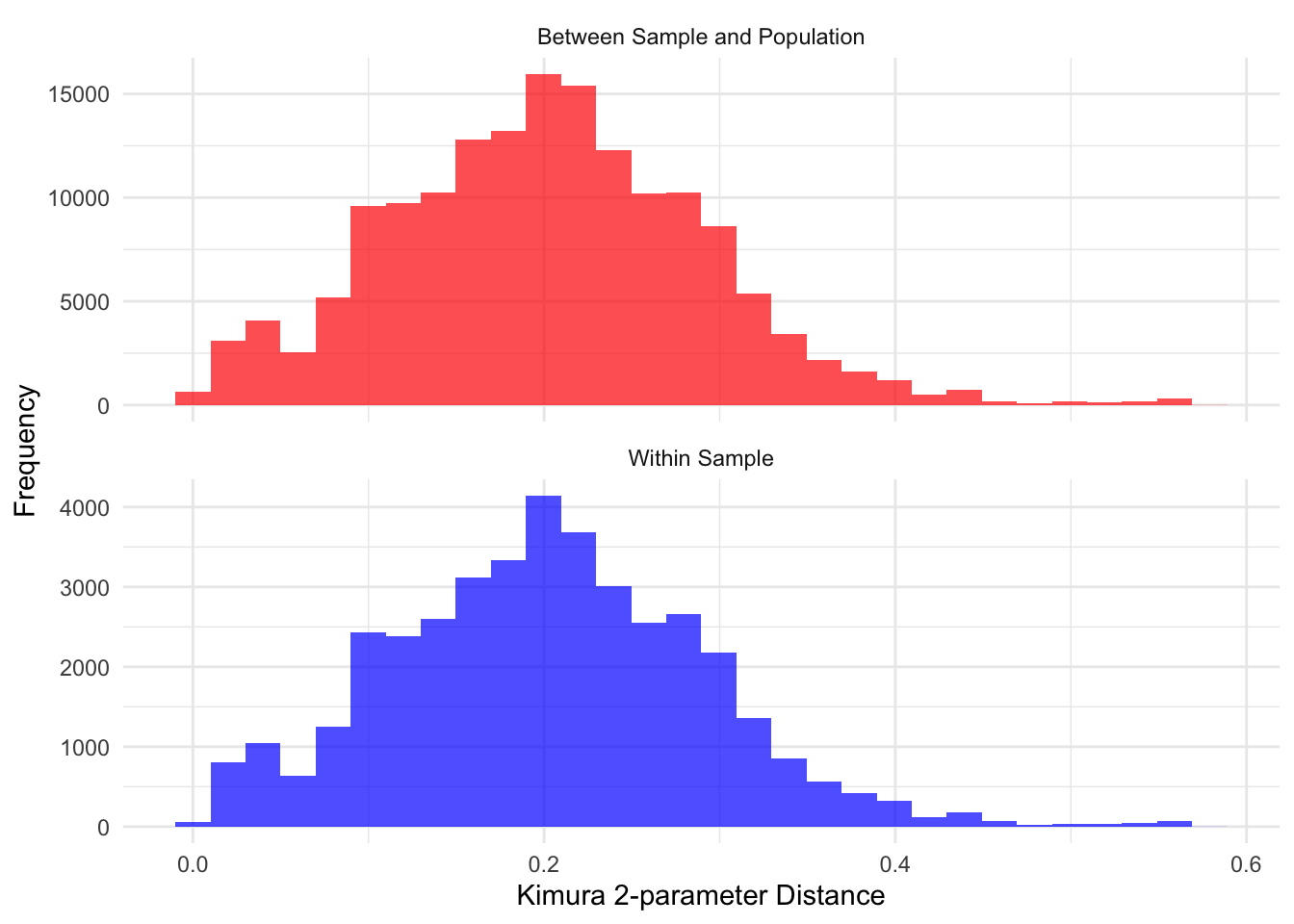

Code

#ggsave("silva_nearest_neighbor_distances_histogram.png", all_distances_df , width = 6, height = 4)

Code

library(gridExtra)
# Function to create histogram without legend or title
create_histogram <- function(data, fill_color) {
  ggplot(data.frame(Distance = data), aes(x = Distance)) +
    geom_histogram(bins = 30, fill = fill_color, alpha = 0.7) +
    labs(# title = "Distribution of Nearest Neighbor Distances",
       x = "Kimura 2-parameter Distance",
       y = "Frequency") +
    theme_minimal() +
    theme(legend.position = "none",
          #axis.title = element_blank(),
          plot.title = element_blank())
}

# Create histograms
hist_within <- create_histogram(unlist(within_sample_distances), "blue")
hist_between <- create_histogram(unlist(between_sample_distances), "red")

# Combine histograms
combined_hist1 <- grid.arrange(hist_within, hist_between, nrow = 2)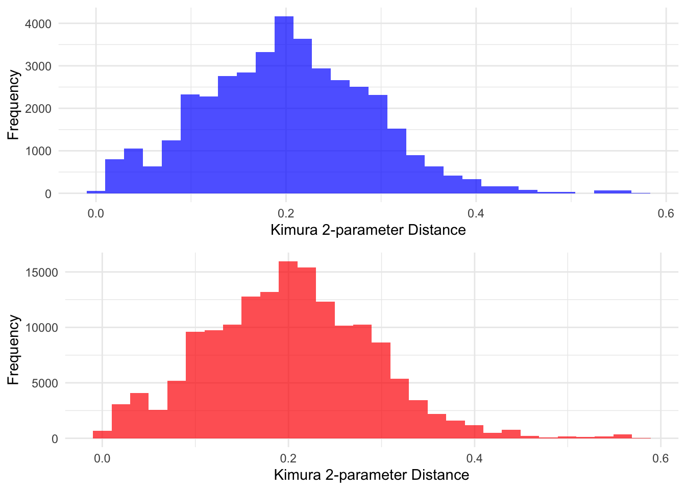

Code

print(combined_hist1)

TableGrob (2 x 1) "arrange": 2 grobs
  z     cells    name           grob
1 1 (1-1,1-1) arrange gtable[layout]
2 2 (2-2,1-1) arrange gtable[layout]

Code

# Save combined histogram
ggsave("silva_combined_distances_histogram.png", combined_hist1, width = 5, height = 5)

Code

# Function to create histogram with density estimate
create_histogram_with_density <- function(data, fill_color, line_color) {
  ggplot(data.frame(Distance = data), aes(x = Distance)) +
    geom_histogram(aes(y = ..density..), bins = 30, fill = fill_color, alpha = 0.7) +
    geom_density(color = line_color, size = 1, alpha = 0.8,adjust=2) +
    theme_minimal() +
    theme(legend.position = "none",
          axis.title = element_blank(),
          plot.title = element_blank())
}

# Create histograms with density estimates
hist_within <- create_histogram_with_density(unlist(within_sample_distances), "blue", "darkblue")
hist_between <- create_histogram_with_density(unlist(between_sample_distances), "red", "darkred")

# Combine histograms
combined_hist2 <- grid.arrange(hist_within, hist_between, nrow = 2)

Code

print(combined_hist2)

TableGrob (2 x 1) "arrange": 2 grobs
  z     cells    name           grob
1 1 (1-1,1-1) arrange gtable[layout]
2 2 (2-2,1-1) arrange gtable[layout]

Code

# Save combined histogram
# ggsave("silva_combined_dist_hist_density.png", combined_hist2, width = 10, height = 5)

Step 4: Using distribution percentiles to find the threshold of “coincidence”

Code

# Assuming within_sample_distances and between_sample_distances are lists of vectors
# Function to calculate percentiles for a list of distance vectors
calculate_percentiles <- function(distance_list, percentiles) {
  all_distances <- unlist(distance_list)
  sapply(percentiles, function(p) quantile(all_distances, p/100))
}

# Calculate 1st and 5th percentiles for both distributions
percentiles <- c(1, 5)
within_percentiles <- calculate_percentiles(within_sample_distances, percentiles)
between_percentiles <- calculate_percentiles(between_sample_distances, percentiles)

# Create a data frame for easy comparison
percentile_comparison <- data.frame(
  Percentile = c("1st", "5th"),
  Within_Sample = within_percentiles,
  Sample_to_Population = between_percentiles
)

# Print the comparison
cat("Comparison of 1st and 5th percentiles:\n")

Comparison of 1st and 5th percentiles:

Code

print(percentile_comparison, row.names = FALSE)

 Percentile Within_Sample Sample_to_Population
        1st    0.01548814           0.01460938
        5th    0.05423807           0.05096344

Code

# Calculate and print the differences
cat("\nDifferences (Within Sample - Sample to Population):\n")


Differences (Within Sample - Sample to Population):

Code

diff_1st <- within_percentiles[1] - between_percentiles[1]
diff_5th <- within_percentiles[2] - between_percentiles[2]
cat("1st percentile difference:", diff_1st, "\n")

1st percentile difference: 0.0008787655

Code

cat("5th percentile difference:", diff_5th, "\n")

5th percentile difference: 0.003274623

Code

# Plot distribution of AD statistics
ad_plot<- ggplot(data.frame(AD_statistic = ad_stats[, "AD_statistic"]), aes(x = AD_statistic)) +
  geom_histogram(aes(y = ..density..), fill = "purple", alpha = 0.7, bins = 30) +
  geom_density(color="purple")+
  geom_density(data = data.frame(stat = ad_stats_null),
               aes(x = stat),
               color = "blue", size = 1) +
  labs(#title = "Distribution of Anderson-Darling Test Statistics",
       x = "AD Statistic",
       y = "Frequency") +
  theme_minimal() +
  theme(legend.position="none",
        plot.title = element_blank())

print(ad_plot)

#ggsave("silva_anderson_darling_histogram.png", ad_plot, width = 5, height = 5)

Code

library(ape)
library(ggplot2)
library(Biostrings)

# Read the aligned sequences
aligned_seqs <- readDNAStringSet("../data/silva_aligned_bacteria_sequences.fasta")

# Take the first 200 sequences
aligned_seqs_200 <- aligned_seqs[1:200]

# Read the sequence information
sequence_info <- read.csv("../data/silva_sequence_info.csv", stringsAsFactors = FALSE)

# Create a named vector for easy lookup
name_mapping <- setNames(sequence_info$original_name, sequence_info$unique_id)

# Convert to DNAbin object (required for dist.dna)
dna_bin <- as.DNAbin(aligned_seqs_200)

# Compute Kimura 2-parameter distances
dist_matrix <- as.matrix(dist.dna(dna_bin, model = "K80", pairwise.deletion = TRUE))

# Function to get unique pairs of sequences with distances smaller than the threshold
get_close_pairs <- function(dist_matrix, threshold) {
  close_pairs <- which(dist_matrix < threshold & dist_matrix > 0 & lower.tri(dist_matrix), arr.ind = TRUE)
  if (nrow(close_pairs) == 0) {
    return(NULL)
  }
  data.frame(
    Seq1 = rownames(dist_matrix)[close_pairs[,1]],
    Seq2 = colnames(dist_matrix)[close_pairs[,2]],
    Distance = dist_matrix[close_pairs]
  )
}

# Set the threshold to 0.015488

threshold <- 0.015488

# Get close pairs
close_pairs_df <- get_close_pairs(dist_matrix, threshold)

if (is.null(close_pairs_df)) {
  cat("No pairs found with distance smaller than", threshold, "\n")
} else {
  cat("Pairs of sequences with distances smaller than", threshold, ":\n\n")
  
  # Print the close pairs with original taxonomic names
  for (i in 1:nrow(close_pairs_df)) {
    cat("Pair", i, ":\n")
    cat("Sequence 1:", name_mapping[close_pairs_df$Seq1[i]], "\n")
    cat("Sequence 2:", name_mapping[close_pairs_df$Seq2[i]], "\n")
    cat("Distance:", close_pairs_df$Distance[i], "\n\n")
  }
  
  cat("Number of unique close pairs found:", nrow(close_pairs_df), "\n")
}

Pairs of sequences with distances smaller than 0.015488 :

Pair 1 :
Sequence 1: Bacteria;Bacillota;Bacilli;Staphylococcales;Staphylococcaceae;Staphylococcus; 
Sequence 2: Bacteria;Bacillota;Bacilli;Staphylococcales;Staphylococcaceae;Staphylococcus; 
Distance: 0.003067494 

Pair 2 :
Sequence 1: Bacteria;Actinomycetota;Actinobacteria;Kitasatosporales;Streptomycetaceae;Streptomyces; 
Sequence 2: Bacteria;Actinomycetota;Actinobacteria;Kitasatosporales;Streptomycetaceae;Streptomyces; 
Distance: 0.01017183 

Pair 3 :
Sequence 1: Bacteria;Actinomycetota;Actinobacteria;Propionibacteriales;Propionibacteriaceae;Cutibacterium; 
Sequence 2: Bacteria;Actinomycetota;Actinobacteria;Propionibacteriales;Propionibacteriaceae;Cutibacterium; 
Distance: 0.01460938 

Pair 4 :
Sequence 1: Bacteria;Actinomycetota;Actinobacteria;Propionibacteriales;Propionibacteriaceae;Cutibacterium; 
Sequence 2: Bacteria;Actinomycetota;Actinobacteria;Propionibacteriales;Propionibacteriaceae;Cutibacterium; 
Distance: 0.01356862 

Pair 5 :
Sequence 1: Bacteria;Cyanobacteriota;Cyanobacteriia;Cyanobacteriales;Coleofasciculaceae;Coleofasciculus PCC-7420; 
Sequence 2: Bacteria;Cyanobacteriota;Cyanobacteriia;Cyanobacteriales;Coleofasciculaceae;Coleofasciculus PCC-7420; 
Distance: 0.01137475 

Number of unique close pairs found: 5

Code

# Histogram of all distances
all_distances <- dist_matrix[lower.tri(dist_matrix)]
ggplot(data.frame(Distance = all_distances), aes(x = Distance)) +
  geom_histogram(bins = 50, fill = "blue", alpha = 0.7) +
  labs(#title = "Distribution of All Pairwise Distances (SILVA)",
       x = "Kimura 2-parameter Distance",
       y = "Frequency") +
  theme_minimal() +
  geom_vline(xintercept = threshold, color = "red", linetype = "dashed")

# Save the histogram
# ggsave("silva_all_distances_histogram.png", width = 10, height = 6)

Code

library(ggplot2)

# Function to create and save the plot
create_ad_plot <- function(p_values, n1, n2, filename) {
  # Calculate 95th and 99th percentiles of the uniform distribution
  percentile_95 <- 0.95
  percentile_99 <- 0.99
  
  p <- ggplot(data.frame(p_value = p_values), aes(x = p_value)) +
    geom_histogram(bins = 30, fill = "skyblue", color = "black", aes(y = ..density..)) +
    geom_hline(yintercept = 1, color = "red", linetype = "dashed") +  # Uniform distribution line
    geom_vline(xintercept = 0.05, color = "red", linetype = "dashed") +
    geom_vline(xintercept = percentile_95, color = "green", linetype = "dashed") +
    geom_vline(xintercept = percentile_99, color = "blue", linetype = "dashed") +
    scale_x_continuous(breaks = c(0, 0.05, percentile_95, percentile_99, 1),
                       labels = c("0", "0.05", "95th", "99th", "1")) +
    labs(x = "Anderson-Darling p-value", 
         y = "Density",
         title = paste("A-D p-values (n1 =", n1, ", n2 =", n2, ")")) +
    theme_minimal() +
    theme(axis.text.x = element_text(angle = 45, hjust = 1))
  
  ggsave(filename, p, width = 8, height = 6)
  
  # Print summary statistics
  cat("For n1 =", n1, "and n2 =", n2, ":\n")
  cat("Proportion of p-values < 0.05:", mean(p_values < 0.05), "\n")
  cat("Mean p-value:", mean(p_values), "\n")
  cat("Median p-value:", median(p_values), "\n\n")
}

# For n1 = 40, n2 = 160
create_ad_plot(ad_results_40_160, 40, 160, "anderson_darling_pvalues_40_160.png")

# For n1 = 100, n2 = 400
# create_ad_plot(ad_results_100_400, 100, 400, "anderson_darling_pvalues_100_400.png")