Prediction set coverage on a real example

Compliance in cholostyramine data

Using the cholostyramine dataset from the bootstrap package

Code

library(bootstrap)  # For the cholost dataset
library(ggplot2)
library(dplyr)
library(gridExtra)
set.seed(20050724)

# Load the cholost dataset
data(cholost)

# Confirm dataset structure
head(cholost)

Code

dim(cholost)  # Should be 164×2

[1] 164   2

Functions to compute the prediction interval

Code

# Function to calculate OLS prediction interval
calculate_pred_interval <- function(X, Y, X_new, alpha = 0.05) {
  n <- nrow(X)
  p <- ncol(X)
  
  # Calculate beta hat
  beta_hat <- solve(t(X) %*% X) %*% t(X) %*% Y
  
  # Calculate fitted values
  Y_hat <- X %*% beta_hat
  
  # Calculate sigma hat squared
  sigma_hat_squared <- sum((Y - Y_hat)^2) / (n - p)
  sigma_hat <- sqrt(sigma_hat_squared)
  
  # Make sure X_new is properly formatted as a row vector
  if(is.vector(X_new)) X_new <- matrix(X_new, nrow=1)
  
  # Calculate prediction for new observation
  Y_pred <- as.numeric(X_new %*% beta_hat)
  
  # Calculate prediction interval width
  pred_var <- sigma_hat_squared * (1 + as.numeric(X_new %*% solve(t(X) %*% X) %*% t(X_new)))
  pred_interval_width <- qnorm(1 - alpha/2) * sqrt(pred_var)
  
  # Return prediction and interval bounds
  return(list(
    prediction = Y_pred,
    lower = Y_pred - pred_interval_width,
    upper = Y_pred + pred_interval_width
  ))
}

Code

# Function for leave-one-out estimate of coverage probability
loo_coverage_probability <- function(X, Y, alpha = 0.05) {
  n <- nrow(X)
  covered <- 0
  
  for (i in 1:n) {
    X_train <- X[-i, , drop = FALSE]
    Y_train <- Y[-i]
    X_test <- matrix(X[i, ], nrow = 1)
    Y_test <- Y[i]
    
    tryCatch({
      pred_interval <- calculate_pred_interval(X_train, Y_train, X_test, alpha)
      if (Y_test >= pred_interval$lower && Y_test <= pred_interval$upper) {
        covered <- covered + 1
      }
    }, error = function(e) {
      cat("Error in LOO iteration", i, ":", e$message, "\n")
    })
  }
  
  return(covered / n)
}

Code

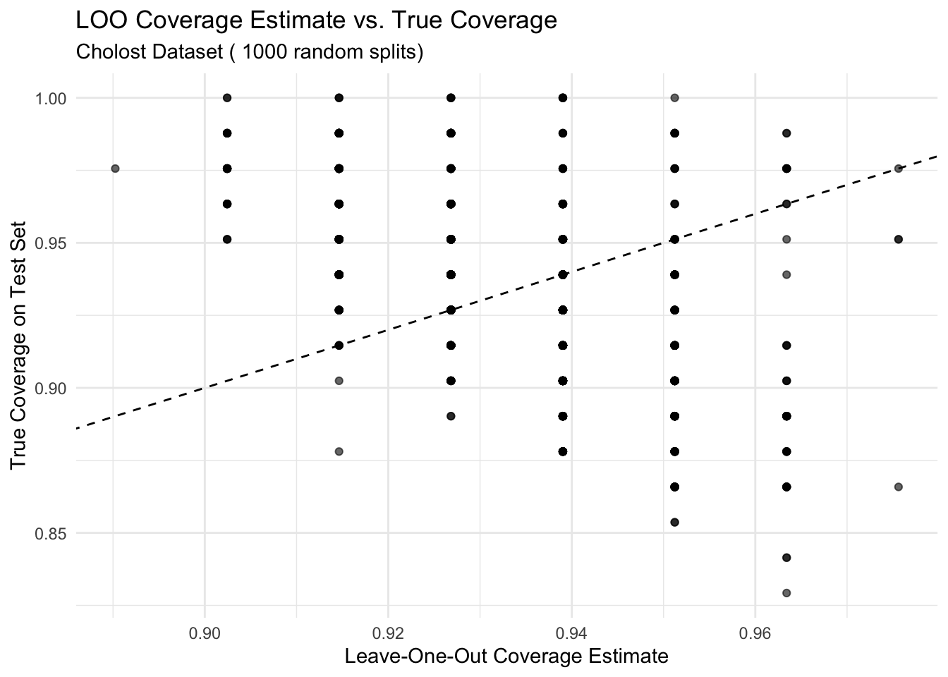
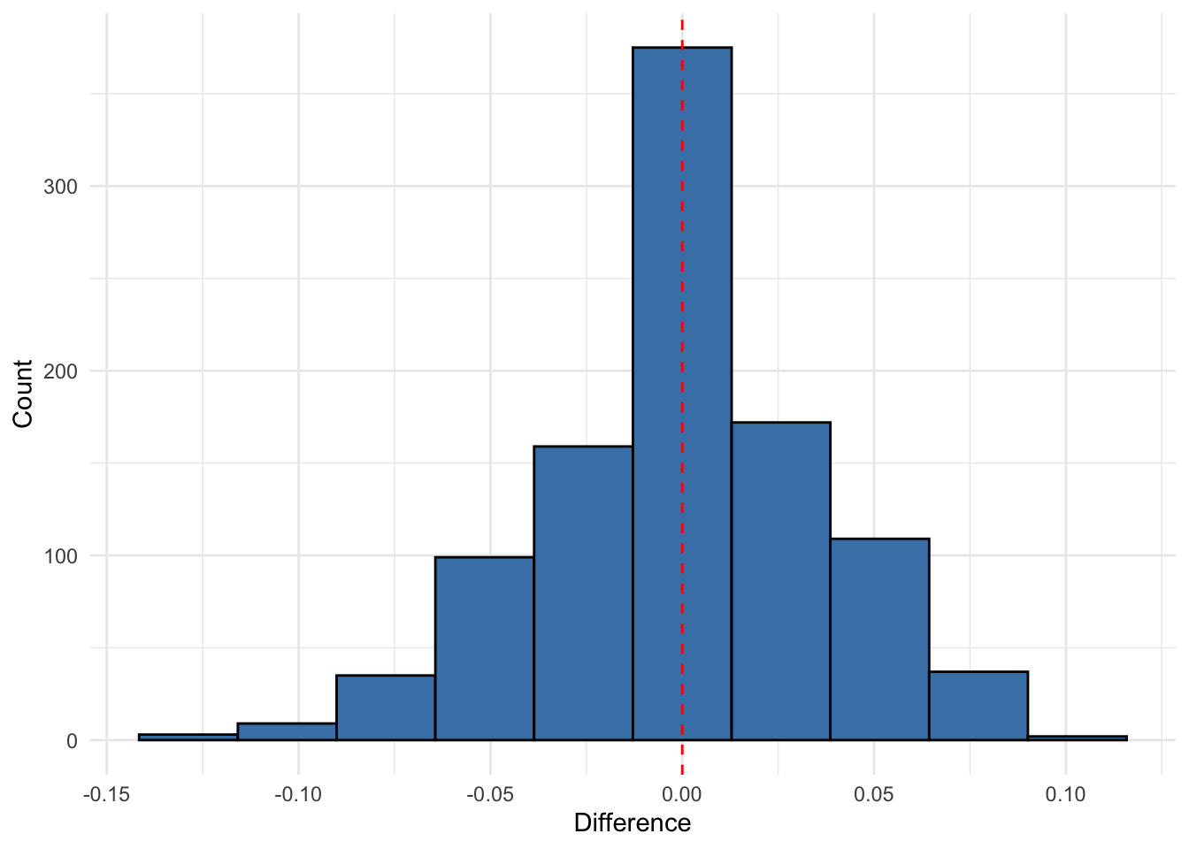
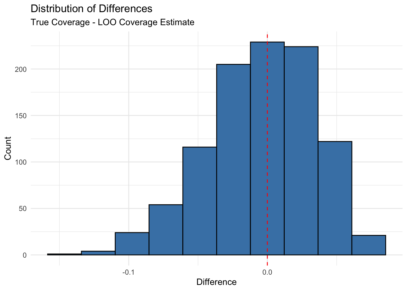
# Prepare the dataset - handling missing values if any
cholost_clean <- na.omit(cholost)

# Define response and predictor
response_var <- "y"  # The response variable
predictor_var <- "z"  # The predictor variable

# Repeat the experiment multiple times to get a distribution of results
n_reps <- 1000
results <- data.frame(
  rep = 1:n_reps,
  true_coverage = numeric(n_reps),
  loo_coverage = numeric(n_reps),
  diff_squared = numeric(n_reps)
)

for (rep in 1:n_reps) {
  # Randomly split the data into training (50%) and test (50%) sets
  n_total <- nrow(cholost_clean)
  train_indices <- sample(1:n_total, size = floor(n_total/2))
  
  train_data <- cholost_clean[train_indices, ]
  test_data <- cholost_clean[-train_indices, ]
  
  # Prepare matrices for training
  X_train <- as.matrix(train_data[, predictor_var, drop = FALSE])
  Y_train <- train_data[[response_var]]
  
  # Prepare matrices for testing
  X_test <- as.matrix(test_data[, predictor_var, drop = FALSE])
  Y_test <- test_data[[response_var]]
  
  # Calculate true coverage on test set
  covered <- 0
  n_test <- nrow(test_data)
  
  for (i in 1:n_test) {
    tryCatch({
      pred_interval <- calculate_pred_interval(X_train, Y_train, X_test[i, , drop = FALSE], alpha = 0.05)
      if (Y_test[i] >= pred_interval$lower && Y_test[i] <= pred_interval$upper) {
        covered <- covered + 1
      }
    }, error = function(e) {
      cat("Error in test coverage calculation, iteration", i, ":", e$message, "\n")
    })
  }
  
  true_cov <- covered / n_test
  
  # Calculate LOO coverage estimate on training set
  loo_cov <- loo_coverage_probability(X_train, Y_train, alpha = 0.05)
  
  # Store results
  results[rep, ] <- c(rep, true_cov, loo_cov, (true_cov - loo_cov)^2)
}

# Calculate average results
avg_results <- summarize(results,
                      mean_true_coverage = mean(true_coverage),
                      mean_loo_coverage = mean(loo_coverage),
                      sd_true_coverage = sd(true_coverage),
                      sd_loo_coverage = sd(loo_coverage),
                      mean_squared_diff = mean(diff_squared))

# Create visualization
p1 <- ggplot(results, aes(x = loo_coverage, y = true_coverage)) +
  geom_point(alpha = 0.6) +
  geom_abline(slope = 1, intercept = 0, linetype = "dashed") +
  labs(title = "LOO Coverage Estimate vs. True Coverage",
       subtitle = paste("Cholost Dataset (", n_reps, "random splits)"),
       x = "Leave-One-Out Coverage Estimate",
       y = "True Coverage on Test Set") +
  theme_minimal()

# Histogram of differences
results$difference <- results$true_coverage - results$loo_coverage
p2 <- ggplot(results, aes(x = difference)) +
  geom_histogram(bins = 10, fill = "steelblue", color = "black") +
  geom_vline(xintercept = 0, linetype = "dashed", color = "red") +
  labs(#title = "Distribution of Differences",
       #subtitle = #"True Coverage - LOO Coverage Estimate",
       x = "Difference",
       y = "Count") +
  theme_minimal()

p2

Code

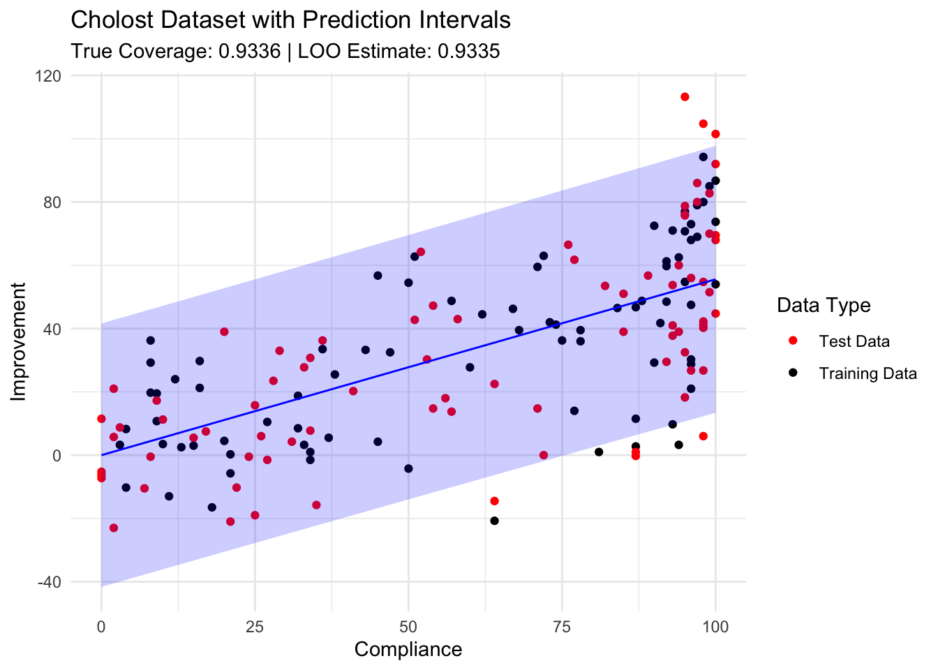
ggsave("histogramdifferences.png",p2,width=6,height=4,bg="white")


# Create a scatter plot with the data and prediction intervals
# (Using one random training set for visualization)
set.seed(44112)
train_indices <- sample(1:nrow(cholost_clean), size = floor(nrow(cholost_clean)/2))
train_data <- cholost_clean[train_indices, ]
test_data <- cholost_clean[-train_indices, ]

X_train <- as.matrix(train_data[, predictor_var, drop = FALSE])
Y_train <- train_data[[response_var]]

# Create a grid of values for z to show the prediction interval
z_grid <- seq(min(cholost_clean$z), max(cholost_clean$z), length.out = 100)
X_grid <- matrix(z_grid, ncol = 1)
predictions <- data.frame(z = z_grid, y_pred = NA, lower = NA, upper = NA)

for (i in 1:length(z_grid)) {
  pred_interval <- calculate_pred_interval(X_train, Y_train, X_grid[i, , drop = FALSE], alpha = 0.05)
  predictions$y_pred[i] <- pred_interval$prediction
  predictions$lower[i] <- pred_interval$lower
  predictions$upper[i] <- pred_interval$upper
}

p3 <- ggplot() +
  geom_point(data = train_data, aes(x = z, y = y, color = "Training Data")) +
  geom_point(data = test_data, aes(x = z, y = y, color = "Test Data")) +
  geom_line(data = predictions, aes(x = z, y = y_pred), color = "blue") +
  geom_ribbon(data = predictions, aes(x = z, ymin = lower, ymax = upper), 
              alpha = 0.2, fill = "blue") +
  scale_color_manual(values = c("Training Data" = "black", "Test Data" = "red")) +
  labs(title = "Cholost Dataset with Prediction Intervals",
       subtitle = paste("True Coverage:", round(mean(results$true_coverage), 4), 
                        "| LOO Estimate:", round(mean(results$loo_coverage), 4)),
        x = "Compliance", y = "Improvement", color = "Data Type") +
  theme_minimal()

# Display plots
#grid.arrange(p1, p2, p3, ncol = 2, layout_matrix = rbind(c(1,2), c(3,3)))

print(p1)

Code

print(p2)

Code

print(p3)

Code

# Print summary statistics
cat("\n--- Summary Statistics ---\n")


--- Summary Statistics ---

Code

print(avg_results)

  mean_true_coverage mean_loo_coverage sd_true_coverage sd_loo_coverage
1          0.9335976         0.9334878       0.03016683       0.0139323
  mean_squared_diff
1       0.001547739

Code

cat("\nMean True Coverage:", round(avg_results$mean_true_coverage, 4))


Mean True Coverage: 0.9336

Code

cat("\nMean LOO Coverage Estimate:", round(avg_results$mean_loo_coverage, 4))


Mean LOO Coverage Estimate: 0.9335

Code

cat("\nMean Squared Difference:", round(avg_results$mean_squared_diff, 6))


Mean Squared Difference: 0.001548

Code

cat("\nStandard Deviation of True Coverage:", round(avg_results$sd_true_coverage, 4))


Standard Deviation of True Coverage: 0.0302

Code

cat("\nStandard Deviation of LOO Coverage:", round(avg_results$sd_loo_coverage, 4))


Standard Deviation of LOO Coverage: 0.0139

Code

# Also fit a standard linear model once to examine the relationship
train_lm <- lm(y ~ z, data = train_data)
summary(train_lm)


Call:
lm(formula = y ~ z, data = train_data)

Residuals:
    Min      1Q  Median      3Q     Max 
-56.387 -12.532   0.995  16.522  39.871 

Coefficients:
            Estimate Std. Error t value Pr(>|t|)    
(Intercept)  0.35902    4.84932   0.074    0.941    
z            0.55122    0.07059   7.809 1.91e-11 ***
---
Signif. codes:  0 '***' 0.001 '**' 0.01 '*' 0.05 '.' 0.1 ' ' 1

Residual standard error: 21.38 on 80 degrees of freedom
Multiple R-squared:  0.4326,    Adjusted R-squared:  0.4255 
F-statistic: 60.98 on 1 and 80 DF,  p-value: 1.91e-11

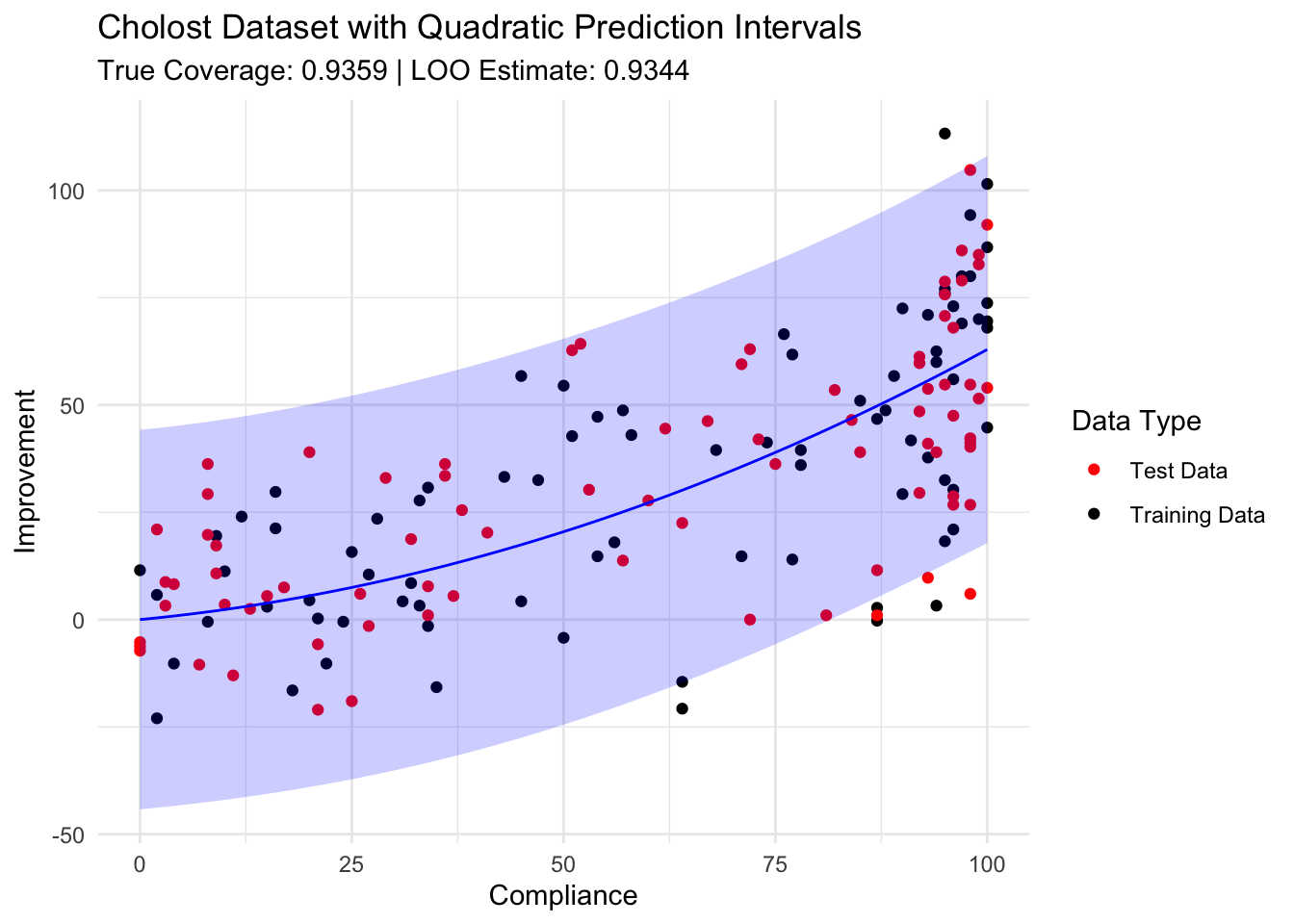
The quadratic version

Code

library(bootstrap)  # For the cholost dataset
library(ggplot2)
library(dplyr)
library(gridExtra)
set.seed(42)

# Load the cholost dataset
data(cholost)

# Confirm dataset structure
head(cholost)

Code

dim(cholost)  # Should be 164×2

[1] 164   2

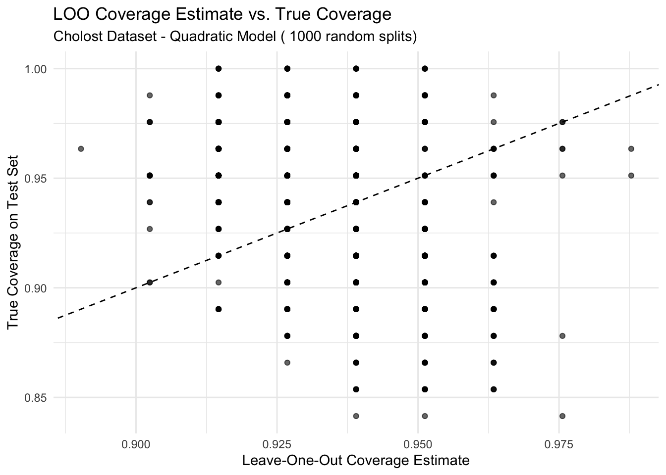
Code

# Function to calculate quadratic regression prediction interval
calculate_quad_pred_interval <- function(X, Y, X_new, alpha = 0.05) {
  # For quadratic regression, we'll add a squared term to the design matrix
  X_quad <- cbind(X, X^2)
  colnames(X_quad) <- c("z", "z_squared")
  
  # For prediction, also square the new X
  X_new_quad <- cbind(X_new, X_new^2)
  
  n <- nrow(X_quad)
  p <- ncol(X_quad)
  
  # Calculate beta hat
  beta_hat <- solve(t(X_quad) %*% X_quad) %*% t(X_quad) %*% Y
  
  # Calculate fitted values
  Y_hat <- X_quad %*% beta_hat
  
  # Calculate sigma hat squared
  sigma_hat_squared <- sum((Y - Y_hat)^2) / (n - p)
  sigma_hat <- sqrt(sigma_hat_squared)
  
  # Calculate prediction for new observation
  Y_pred <- as.numeric(X_new_quad %*% beta_hat)
  
  # Calculate prediction interval width
  pred_var <- sigma_hat_squared * (1 + as.numeric(X_new_quad %*% solve(t(X_quad) %*% X_quad) %*% t(X_new_quad)))
  pred_interval_width <- qnorm(1 - alpha/2) * sqrt(pred_var)
  
  # Return prediction and interval bounds
  return(list(
    prediction = Y_pred,
    lower = Y_pred - pred_interval_width,
    upper = Y_pred + pred_interval_width
  ))
}

# Function for leave-one-out estimate of coverage probability with quadratic regression
loo_coverage_probability <- function(X, Y, alpha = 0.05) {
  n <- nrow(X)
  covered <- 0
  
  for (i in 1:n) {
    X_train <- X[-i, , drop = FALSE]
    Y_train <- Y[-i]
    X_test <- matrix(X[i, ], nrow = 1)
    Y_test <- Y[i]
    
    tryCatch({
      pred_interval <- calculate_quad_pred_interval(X_train, Y_train, X_test, alpha)
      if (Y_test >= pred_interval$lower && Y_test <= pred_interval$upper) {
        covered <- covered + 1
      }
    }, error = function(e) {
      cat("Error in LOO iteration", i, ":", e$message, "\n")
    })
  }
  
  return(covered / n)
}

# Prepare the dataset - handling missing values if any
cholost_clean <- na.omit(cholost)

# Define response and predictor
response_var <- "y"  # The response variable
predictor_var <- "z"  # The predictor variable

# Repeat the experiment multiple times to get a distribution of results
n_reps <- 1000
results <- data.frame(
  rep = 1:n_reps,
  true_coverage = numeric(n_reps),
  loo_coverage = numeric(n_reps),
  diff_squared = numeric(n_reps)
)

for (rep in 1:n_reps) {
  # Randomly split the data into training (50%) and test (50%) sets
  n_total <- nrow(cholost_clean)
  train_indices <- sample(1:n_total, size = floor(n_total/2))
  
  train_data <- cholost_clean[train_indices, ]
  test_data <- cholost_clean[-train_indices, ]
  
  # Prepare matrices for training
  X_train <- as.matrix(train_data[, predictor_var, drop = FALSE])
  Y_train <- train_data[[response_var]]
  
  # Prepare matrices for testing
  X_test <- as.matrix(test_data[, predictor_var, drop = FALSE])
  Y_test <- test_data[[response_var]]
  
  # Calculate true coverage on test set
  covered <- 0
  n_test <- nrow(test_data)
  
  for (i in 1:n_test) {
    tryCatch({
      pred_interval <- calculate_quad_pred_interval(X_train, Y_train, X_test[i, , drop = FALSE], alpha = 0.05)
      if (Y_test[i] >= pred_interval$lower && Y_test[i] <= pred_interval$upper) {
        covered <- covered + 1
      }
    }, error = function(e) {
      cat("Error in test coverage calculation, iteration", i, ":", e$message, "\n")
    })
  }
  
  true_cov <- covered / n_test
  
  # Calculate LOO coverage estimate on training set
  loo_cov <- loo_coverage_probability(X_train, Y_train, alpha = 0.05)
  
  # Store results
  results[rep, ] <- c(rep, true_cov, loo_cov, (true_cov - loo_cov)^2)
}

# Calculate average results
avg_results <- summarize(results,
                      mean_true_coverage = mean(true_coverage),
                      mean_loo_coverage = mean(loo_coverage),
                      sd_true_coverage = sd(true_coverage),
                      sd_loo_coverage = sd(loo_coverage),
                      mean_squared_diff = mean(diff_squared))

# Create visualization
p1 <- ggplot(results, aes(x = loo_coverage, y = true_coverage)) +
  geom_point(alpha = 0.6) +
  geom_abline(slope = 1, intercept = 0, linetype = "dashed") +
  labs(title = "LOO Coverage Estimate vs. True Coverage",
       subtitle = paste("Cholost Dataset - Quadratic Model (", n_reps, "random splits)"),
       x = "Leave-One-Out Coverage Estimate",
       y = "True Coverage on Test Set") +
  theme_minimal()

# Histogram of differences
results$difference <- results$true_coverage - results$loo_coverage
p2 <- ggplot(results, aes(x = difference)) +
  geom_histogram(bins = 10, fill = "steelblue", color = "black") +
  geom_vline(xintercept = 0, linetype = "dashed", color = "red") +
  labs(title = "Distribution of Differences",
       subtitle = "True Coverage - LOO Coverage Estimate",
       x = "Difference",
       y = "Count") +
  theme_minimal()

# Create a scatter plot with the data and prediction intervals
# (Using one random training set for visualization)
set.seed(123)
train_indices <- sample(1:nrow(cholost_clean), size = floor(nrow(cholost_clean)/2))
train_data <- cholost_clean[train_indices, ]
test_data <- cholost_clean[-train_indices, ]

X_train <- as.matrix(train_data[, predictor_var, drop = FALSE])
Y_train <- train_data[[response_var]]

# Create a grid of values for z to show the prediction interval
z_grid <- seq(min(cholost_clean$z), max(cholost_clean$z), length.out = 100)
X_grid <- matrix(z_grid, ncol = 1)
predictions <- data.frame(z = z_grid, y_pred = NA, lower = NA, upper = NA)

for (i in 1:length(z_grid)) {
  pred_interval <- calculate_quad_pred_interval(X_train, Y_train, X_grid[i, , drop = FALSE], alpha = 0.05)
  predictions$y_pred[i] <- pred_interval$prediction
  predictions$lower[i] <- pred_interval$lower
  predictions$upper[i] <- pred_interval$upper
}

p3 <- ggplot() +
  geom_point(data = train_data, aes(x = z, y = y, color = "Training Data")) +
  geom_point(data = test_data, aes(x = z, y = y, color = "Test Data")) +
  geom_line(data = predictions, aes(x = z, y = y_pred), color = "blue") +
  geom_ribbon(data = predictions, aes(x = z, ymin = lower, ymax = upper), 
              alpha = 0.2, fill = "blue") +
  scale_color_manual(values = c("Training Data" = "black", "Test Data" = "red")) +
  labs(title = "Cholost Dataset with Quadratic Prediction Intervals",
       subtitle = paste("True Coverage:", round(mean(results$true_coverage), 4), 
                        "| LOO Estimate:", round(mean(results$loo_coverage), 4)),
       x = "Compliance", y = "Improvement", color = "Data Type") +
  theme_minimal()

# Display plots
#grid.arrange(p1, p2, p3, ncol = 2, layout_matrix = rbind(c(1,2), c(3,3)))

print(p1)

Code

print(p2)

Code

print(p3)

Code

# Print summary statistics
cat("\n--- Summary Statistics ---\n")


--- Summary Statistics ---

Code

print(avg_results)

  mean_true_coverage mean_loo_coverage sd_true_coverage sd_loo_coverage
1          0.9358902         0.9344268       0.03171133       0.0135256
  mean_squared_diff
1        0.00148602

Code

cat("\nMean True Coverage:", round(avg_results$mean_true_coverage, 4))


Mean True Coverage: 0.9359

Code

cat("\nMean LOO Coverage Estimate:", round(avg_results$mean_loo_coverage, 4))


Mean LOO Coverage Estimate: 0.9344

Code

cat("\nMean Squared Difference:", round(avg_results$mean_squared_diff, 6))


Mean Squared Difference: 0.001486

Code

cat("\nStandard Deviation of True Coverage:", round(avg_results$sd_true_coverage, 4))


Standard Deviation of True Coverage: 0.0317

Code

cat("\nStandard Deviation of LOO Coverage:", round(avg_results$sd_loo_coverage, 4))


Standard Deviation of LOO Coverage: 0.0135

Code

# Also fit a standard quadratic model once to examine the relationship
train_quad <- lm(y ~ z + I(z^2), data = train_data)
summary(train_quad)


Call:
lm(formula = y ~ z + I(z^2), data = train_data)

Residuals:
    Min      1Q  Median      3Q     Max 
-53.568 -13.064   3.445  17.227  55.313 

Coefficients:
             Estimate Std. Error t value Pr(>|t|)  
(Intercept)  5.458842   8.232416   0.663    0.509  
z           -0.019853   0.364572  -0.054    0.957  
I(z^2)       0.006024   0.003207   1.878    0.064 .
---
Signif. codes:  0 '***' 0.001 '**' 0.01 '*' 0.05 '.' 0.1 ' ' 1

Residual standard error: 22.64 on 79 degrees of freedom
Multiple R-squared:  0.4941,    Adjusted R-squared:  0.4813 
F-statistic: 38.58 on 2 and 79 DF,  p-value: 2.046e-12